The Sharpe Stability Ratio: Evaluating the Sharpe Ratio Temporal Consistency

The Sharpe Ratio¹, one of the most commonly used measure of risk-adjusted performance², is usually reported as a point estimate (Morningstar, Quantalys, etc.).

Thanks to the work of Lo³, Opdyke⁴ and more recently⁵ de Prado et al.⁶, it is nevertheless well understood that such a point estimate […] does not convey information about statistical significance⁶, so that a more meaningful way to measure and compare investment efficiency⁶ is rather to report the Probabilistic Sharpe Ratio (PSR)⁷, which expresses observed Sharpe Ratios in probability space, adjusting for skewness, kurtosis, serial correlation, and sample length⁶.

However, these two measures cannot distinguish persistent skill from episodic outperformance⁸ because they both evaluate performance at a single temporal aggregation without quantifying how risk-adjusted returns evolve within the sample period⁸.

In order to overcome this limitation, Traver and Rodriguez Dominguez⁸ introduces the Sharpe Stability Ratio⁸, a measure of the temporal consistency of the Sharpe Ratio across overlapping subperiods.

In this blog post, I will first describe the Sharpe Stability Ratio in details and then, as examples of usage, I will:

• Show that it provides additional information compared to the Sharpe Ratio
• Show that it also provides additional information compared to another measure of risk-adjusted performances called the Ulcer Performance Index⁹
• Experiment with it as a portfolio optimization objective and construct its associated efficient frontier

Reminders

The Sharpe Ratio

Let be:

• $r_1,…,r_T$ the observed arithmetic returns of an investment (asset/fund/portfolio/trading strategy/etc.) over $T$ periods of time
• $r_{f,1},…,r_{f,T}$, the observed risk-free arithmetic returns¹⁰ over the same $T$ periods of time
• $ r_1 - r_{f,1},…,r_T - r_{f,T}$, the associated investment observed excess arithmetic returns over the risk-free rate

Then, the observed Sharpe Ratio¹ $\widehat{SR}$ of the investment over the period $1..T$ is defined as:

\[\widehat{SR} = \frac{\widehat{\mu}_{r - r_f}}{\widehat{\sigma}_{r - r_f}}\]

, where:

• $\widehat{\mu}_{r - r_f}$ is the sample mean of the excess arithmetic returns
• $\widehat{\sigma}_{r - r_f}^2$ is the sample¹¹ variance of the excess arithmetic returns

The Sharpe Ratio provides a scale-free summary of expected excess return per unit of risk⁸ and can be interpreted as a measure of […] signal over noise, or skill over luck⁶.

Prado et al.⁶ notes that the Sharpe ratio satisfies several important properties⁶, among which:

• It is rooted in Markowitz’s mean-variance analysis model.

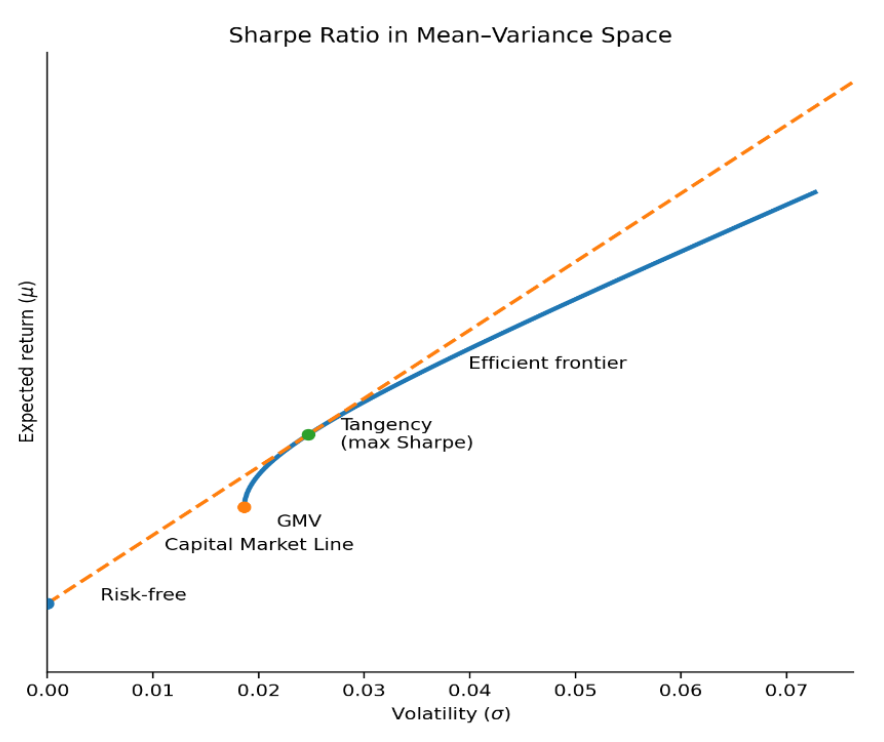
  For example, as illustrated in Figure 1, the tangency portfolio is the mean-variance efficient portfolio with maximum Sharpe Ratio and all efficient portfolios are linear combinations of this portfolio and the risk-free asset¹².

  

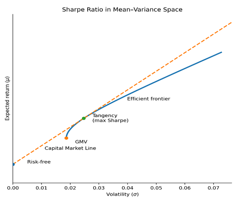
  Figure 1. The Sharpe Ratio in Mean-Variance Space. Source: de Prado.

  As another example, ranking portfolios by their Sharpe Ratios yields the same ordering as expected-utility maximization⁶ under three (sufficient) conditions:

  • When portfolio returns follow a normal, or more generally an elliptical distribution
  • When portfolio returns satisfy the LS property¹³, that is, when portfolio returns differ from one another only by location and scale parameters¹³
  • When investor preferences admit a mean–variance representation, either exactly or as a second-order approximation⁶

  
  

• It is actually well defined and usable for any return process with finite mean and variance, regardless of higher-order moments or temporal dependence⁶.

  This property is of practical importance because a common misunderstanding regarding [the Sharpe Ratio] is that […] [its users] must implicitly assume that returns are i.i.d. Normal⁶.

  As explained in de Prado et al.⁶, this is incorrect:

  When returns are non-normal or serially correlated, variance may no longer fully characterize downside or tail risk, but it continues to measure dispersion, and the Sharpe Ratio retains its economic interpretation as expected excess return per unit of standard deviation.

  Moreover, while several alternative risk-adjusted performance measures have been proposed over the years - whether partial moments-based (Sortino Ratio, Omega Ratio…), drawdown-based (Calmar Ratio…) or Value-at-Risk-based (Rachev Ratio…) - empirical studies have regularly shown that portfolio rankings based on most¹⁴ of these measures are nearly identical to those determined by the Sharpe ratio¹³.

  This behavior is partially explained in Schuhmacher and Elingby¹³, which demonstrates that if portfolio returns satisfy the LS property¹⁵, then any “reasonable” risk-adjusted performance measure must be a strictly increasing function in the Sharpe ratio¹³.

The Probabilistic Sharpe Ratio

The usage of hats in the previous subsection for the definition of the Sharpe Ratio emphasises that $\widehat{\mu}_{r - r_f}$ , $\widehat{\sigma}_{r - r_f}^2$ and $\widehat{SR}$ are quantities computed from the observed excess returns $r_1 - r_{f,1}$,…,$r_T - r_{f,T}$ while the true mean excess return $\mu_{r - r_f}$, the true variance $\sigma_{r - r_f}^2$ and the true Sharpe ratio $ SR = \frac{\mu_{r - r_f}}{\sigma_{r - r_f}} $ are quantities associated with the unobservable excess return generating process.

It follows that the observed Sharpe Ratio $\widehat{SR}$ is a statistical estimator of its true counterpart $SR$, subject to an estimation error quantified by Lo³, Opdyke⁴ and de Prado et al.⁶ under various assumptions on the excess return generating process¹⁶.

In order for practitioners to evaluate the credibility of [an] observed Sharpe Ratio⁸ without explicitely referring to the underlying statistical machinery¹⁷, Bailey and de Prado⁷ introduces the Probabilistic Sharpe Ratio $\widehat{PSR}(SR_0)$, a risk-adjusted performance measure defined as the probability that the Sharpe Ratio estimator $\widehat{SR}$ is greater than a benchmark Sharpe Ratio $SR_0$¹⁸ over the period $1..T$:

\[\widehat{PSR}(SR_0) = \Phi\left( \frac{\widehat{SR} - SR_0}{ \sqrt{\frac{1 - \widehat{\kappa}_{r - r_f} \widehat{SR} + (\widehat{\gamma}_{r - r_f} - 1) \frac{\widehat{SR}^2}{4}}{T}} } \right )\]

, where:

• $\kappa_{r - r_f}$ and $\gamma_{r - r_f}$ are the true skewness and the true kurtosis of the unobservable excess return generating process and $\widehat{\kappa}_{r - r_f}$ and $\widehat{\gamma}_{r - r_f}$ their empirical counterparts
• $\Phi$ is the cumulative distribution function of the standard normal distribution

This makes the Probabilistic Sharpe Ratio one of the very few¹⁹ alternative risk-adjusted performance measures that explicitly penalizes uncertainty due to short samples, downside, tail and drawdown-related risks⁶ while still being grounded in modern portfolio theory⁶.

As a side note, de Prado et al.⁶ further improves the Probabilistic Sharpe Ratio by taking into account the return generating process’s autocorrelation, which enables Sharpe Ratio inference under substantially more general assumptions than prior closed-form treatments⁶, including the original treatment in Bailey and de Prado⁷.

The Sharpe Stability Ratio

Definition

Traver and Rodriguez Dominguez⁸ notes that neither the Sharpe Ratio nor the Probabilistic Sharpe Ratio enables statistical inference on temporal stability of risk-adjusted performance⁸, because they are both risk-adjusted performance measures computed over the full period $1..T$.

Naturally, practitioners routinely compute rolling Sharpe Ratios to visualize [risk-adjusted performance] dynamics⁸, but no formal framework exists for statistical inference on temporal stability when these rolling estimates are constructed from overlapping windows that induce autocorrelation⁸.

To resolve this shortcoming, Traver and Rodriguez Dominguez⁸ introduces the Sharpe Stability Ratio $\widehat{SSR}(SR_0)$, defined as the mean rolling Sharpe Ratio minus a benchmak Sharpe Ratio $SR_0$¹⁸ divided by its long-run (or asymptotic²⁰) standard deviation:

\[\widehat{SSR}(SR_0) = \frac{\widehat{\mu}_{\hat{z}} - SR_0}{\widehat{\sigma}_{\infty, \hat{z}}}\]

, where:

• $\hat{z}_1 = \widehat{SR}_{1:w}$, $\hat{z}_2 = \widehat{SR}_{2:w+1}$, …, $\hat{z}_{T-w+1} = \widehat{SR}_{T-w+1:T}$ are the Sharpe Ratios over the time periods $1..w$, $2..w+1$, …, $T-w+1…T$

  Here, because the time periods $1..w$, $2..w+1$, …, $T-w+1…T$ are overlapping, the associated Sharpe Ratios $\hat{z}_1$, $\hat{z}_2$, …, $\hat{z}_{T-w+1}$ are usually called rolling Sharpe Ratios.

• $\widehat{\mu}_{\hat{z}} = \frac{1}{T-w+1} \sum_{k=1}^{T-w+1} \hat{z}_k$ is the sample mean of the rolling Sharpe Ratios $\hat{z}_1$, $\hat{z}_2$, …, $\hat{z}_{T-w+1}$

• $\widehat{\sigma}_{\infty, \hat{z}}^2$ is an estimator of the long-run variance of the rolling Sharpe Ratios $\hat{z}_1$, $\hat{z}_2$, …, $\hat{z}_{T-w+1}$

  Contrary to the standard variance $\sigma^2$, the long-run variance $\sigma^2_{\infty}$ is a measure of uncertainty in the mean that accounts for serial correlation.

  In the specific case of the Sharpe Stability Ratio, using the long-run variance instead of the variance is made necessary by⁸:

  • The usage of overlapping windows in the computation of the rolling Sharpe Ratios $\hat{z}_1$, $\hat{z}_2$, …, $\hat{z}_{T-w+1}$

    Indeed, successive windows share $w-1$ observations, implying first-order autocorrelation close to one when $w$ is large relative to the sampling frequency⁸, which would lead the naive variance estimator [to understate] the long-run variance by a factor of order $w$⁸.

  • The (potential) serial dependence in the excess returns $ r_1 - r_{f,1},…,r_T - r_{f,T}$

  As a practical estimator for $\sigma^2_{\infty}$, Traver and Rodriguez Dominguez⁸ chooses the Newey–West heteroskedasticity and autocorrelation consistent (HAC) estimator²⁰ with the triangular kernel, also known as the Bartlett kernel²¹:

  \[\widehat{\sigma}_{\infty, \hat{z}}^2 = \widehat{\gamma}_{0, \hat{z}} + 2 \sum_{k=1}^L \left( 1 - \frac{k}{L + 1} \right) \widehat{\gamma}_{k, \hat{z}}\]

  , where:

  • $\widehat{\gamma}_{0, \hat{z}}$ is equal to the sample variance of the rolling Sharpe Ratios, that is, $\frac{1}{T-w+1} \sum_{k=1}^{T-w+1} \left( \hat{z}_k - \widehat{\mu}_{\hat{z}} \right)^2$
  • $\widehat{\gamma}_{k, SRs}, k \geq 1$ is equal to the sample autocovariance of the rolling Sharpe Ratios at lag $k$, that is, $ \frac{1}{T-w+1} \sum_{t=k+1}^{T-w+1} \left( \hat{z}_t - \widehat{\mu}_{\hat{z}} \right) \left( \hat{z}_{t-k} - \widehat{\mu}_{\hat{z}} \right) $
  • $L \geq 0$ is a lag truncation parameter, estimated by the nonparametric data-dependent procedure of Newey and West²² based on both theoretical asymptotic and empirical Monte Carlo results²²

Interpretation

Similar to the Sharpe Ratio that is a signal-to-noise ratio for the excess returns $ r_1 - r_{f,1},…,r_T - r_{f,T}$, the Sharpe Stability Ratio is by definition a signal-to-noise ratio for the rolling Sharpe Ratios $\hat{z}_1$, $\hat{z}_2$, …, $\hat{z}_{T-w+1}$.

In terms of values:

• A strongly positive Sharpe Stability Ratio is desirable because it indicates stable superior performances v.s. the benchmark
• Conversely, a strongly negative Sharpe Stability Ratio is usually not desirable because it indicates stable inferior performances v.s. the benchmark
• Last, a zero-ish Sharpe Stability Ratio is usually not desirable either because it typically indicates instability of performances²³ - whether positive of negative - v.s. the benchmark

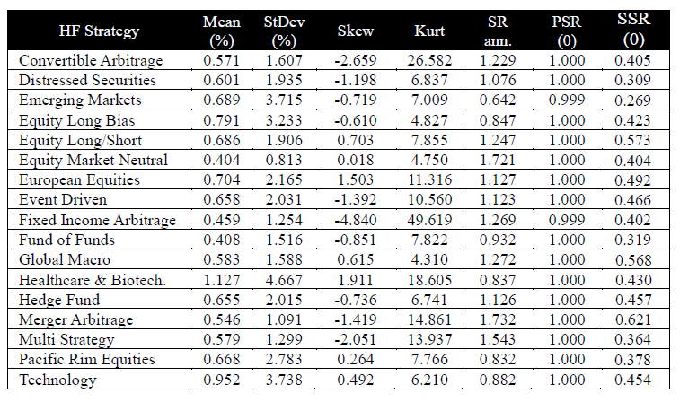
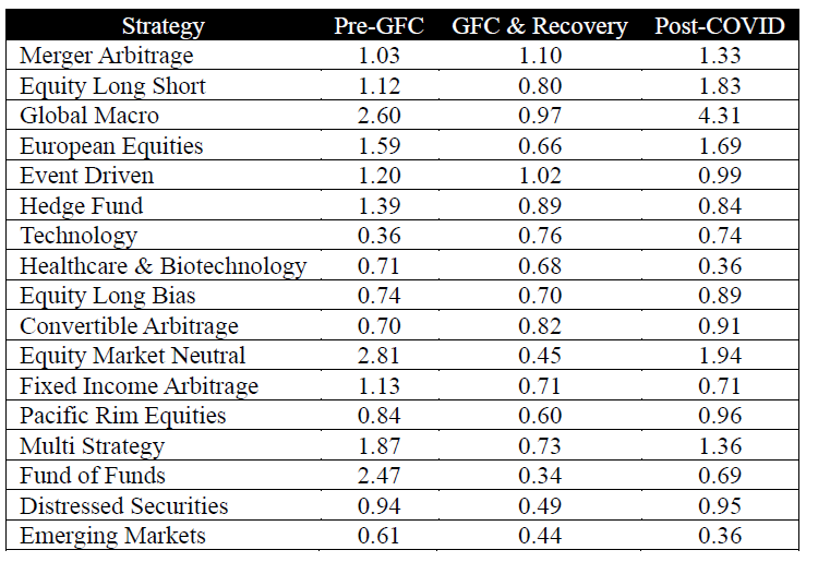
A handful of reference values for 17 Barclay Hedge Fund Indices, representing real-world strategies with pronounced non-normality, serial dependence and regime-switching behavior⁸, are provided in Traver and Rodriguez Dominguez⁸.

For convenience, they are reproduced in Figure 2 (full sample analysis) and Figure 3 (subperiods analysis).

Figure 2. Misc. statistics inc. SSR(0) over the full period, 17 Barclay Hedge Hedge Fund strategy indices, January 1997 - December 2025. Source: Traver and Rodriguez Dominguez.

Figure 3. Analysis of SSR(0) over subperiods, 17 Barclay Hedge Hedge Fund strategy indices, January 1997 - December 2025. Source: Traver and Rodriguez Dominguez.

Two comments from these figures:

• It seems that reaching a Sharpe Stability Ratio of 1 is challenging but achievable²⁴, so that this value could be considered as a (high) reference value to have in mind when interpreting Sharpe Stability Ratios.

  By extension, an interesting question is how high a Sharpe Stability Ratio could be or could not be?

  To answer that question, I propose to use Bernard Madoff’s Fairfield Sentry fund.

  Because it is now established that this fund was a fraud, studying it generally helps to find implausible risk-adjusted performance metrics.

  Figure 4 compares the performance of the S&P500 to that of the Fairfield Sentry fund²⁵ over a little less than 20 years.

  

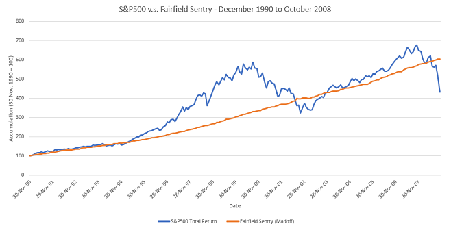
  Figure 4. S&P500 v.s. Fairfield Sentry, November 1990 - October 2008.

  Using 36 months²⁶ as a rolling window length for the Sharpe Stability Ratio computation, figures are provided below.

  Instrument	Monthly Sharpe Ratio (0)	Probabilistic Sharpe Ratio (0)	Sharpe Stability Ratio (0)
  S&P500 (Total Return)	0.19	0.99	0.37
  Fairfield Sentry fund	1.19	1	1.55

  From this table, an investment exhibiting a Sharpe Stability Ratio of about 1.5 over a 20-year period should then be considered as highly suspicious.

  Now, it is possible to go a little further and compute the Sharpe Stability Ratio of the Fairfield Sentry fund on an expanding window basis²⁷, which will provide reference values for an implausible Sharpe Stability Ratio over all standard evaluation periods for an investment.

  Results are provided in Figure 5, on which the apparently huge Sharpe Stability Ratio of 4.31 reported for the Global Macro Hedge Fund Strategy Indice (Figure 3) is not so huge anymore when compared to the Sharpe Stability Ratio of 12 computed for the airfield Sentry fund over an equivalent period of 5 years!

  

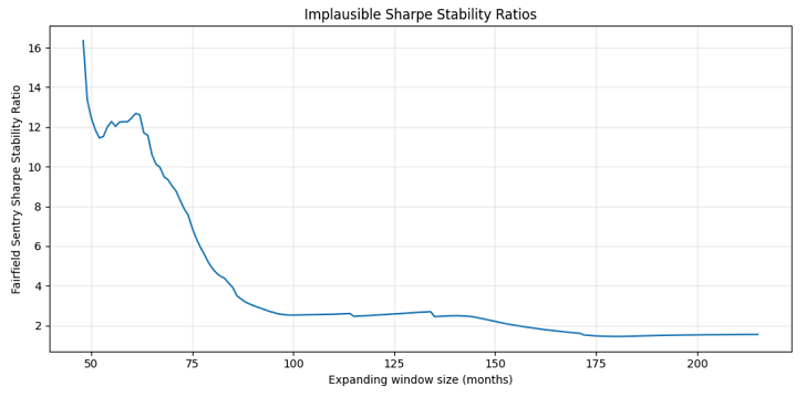
  Figure 5. Fairfield Sentry Sharpe Stability Ratio, expanding window from November 1994 to October 2008.

• Temporal stability, as measured by [the Sharpe Stability Ratio], is inherently conditional on the prevailing market regime rather than an intrinsic, regime-invariant attribute of each strategy⁸.

  As a consequence, the Sharpe Stability Ratio also captures how consistently a strategy performs within a given macro-financial environment and how its stability profile shifts across environments⁸.

Asymptotic distribution and statistical inference

Traver and Rodriguez Dominguez⁸ establishes that under stationarity and $\alpha$-mixing assumptions, the Sharpe Stability Ratio satisfies

\[\sqrt{T-w+1} \widehat{SSR}(SR_0) \overset{a}{\sim} N \left( 0, 1 \right)\]

That asymptotic normality provides a theoretical basis for making inference about the Sharpe Stability Ratio, although Traver and Rodriguez Dominguez⁸ emphasises that in practice, due to the strong autocorrelation induced by overlapping windows⁸, bootstrap inference should be prefered to asymptotic approximations.

A couple more words on asymptotic results, though.

If we introduce the “normalized” Sharpe Stability Ratio $\widehat{nSSR}(SR_0)$ defined by

\[\widehat{nSSR}(SR_0) = \sqrt{T-w+1} \widehat{SSR}(SR_0)\]

, it then becomes possible to interpret the associated (normalized) Sharpe Stability Ratio values in statistical terms, which might be useful to become familiar with this new risk-adjusted performance measure.

For example:

• A normalized Sharpe Stability Ratio value of about 1.96 would imply that $SR_0$ lies inside the 95% confidence interval around the mean rolling Sharpe Ratio
• A normalized Sharpe Stability Ratio value of about 2.576 would imply that $SR_0$ lies inside the 99% confidence interval around the mean rolling Sharpe Ratio

As other examples:

• A strongly positive normalized Sharpe Stability Ratio value would imply that the mean rolling Sharpe Ratio is substantially greater than $SR_0$
• A strongly negative normalized Sharpe Stability Ratio value would imply that the mean rolling Sharpe Ratio is substantially lower than $SR_0$
• A normalized Sharpe Stability Ratio value close to zero would imply that the mean rolling Sharpe Ratio is close to $SR_0$

Comparison with other Sharpe Ratio-based measures

With the introduction of the Sharpe Stability Ratio, there are now at least²⁸ 3 Sharpe Ratio-based risk-adjusted performance measures to choose from when analyzing an investment:

• The Sharpe Ratio
• The Probabilistic Sharpe Ratio
• The Sharpe Stability Ratio

Figure 6 summarizes the main question answered by each of these measures.

Figure 6. Different Sharpe Ratio Dimensions: SR, PSR, SSR. Source: Traver and Rodriguez Dominguez.

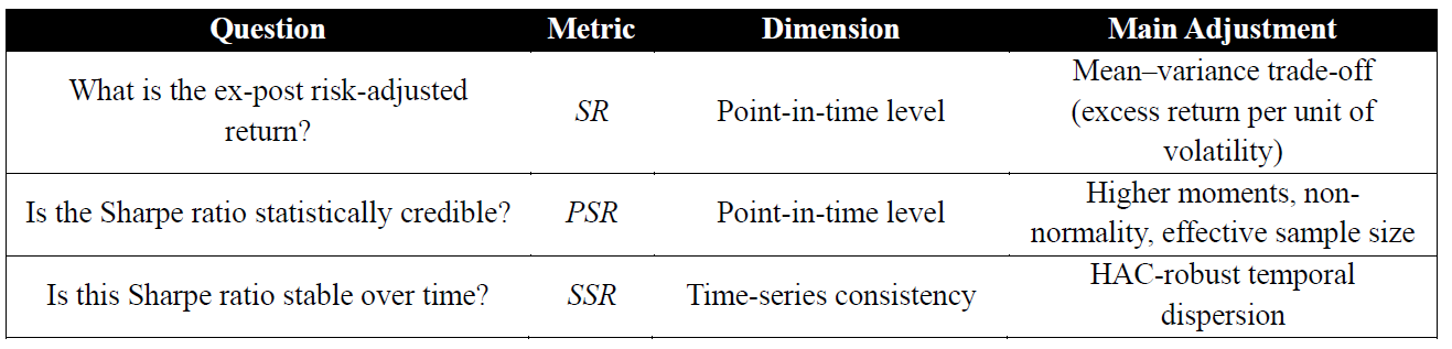
As can be seen in Figure 6, each of these measures capture a different dimension of performance evaluation⁸.

Among them, the Sharpe Stability Ratio focuses on the persistence of risk-adjusted performances over time, which allows it to distinguish between investments with a similar Sharpe Ratio and Probabilistic Sharpe Ratio.

As an example, Figure 7 represents 3 different synthetic strategies with the same²⁹ Sharpe Ratios and Probabilistic Sharpe Ratios but different Sharpe Stability Ratios.

Figure 7. Three synthetic strategies with identical Sharpe Ratios and Probabilistic Sharpe Ratios (0, 0.5 and 1.0). Source: Traver and Rodriguez Dominguez.

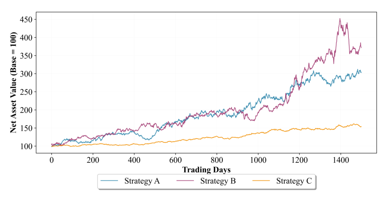
From a visual inspection of Figure 7, Strategy A would be the preferred strategy in terms of temporal stability, which is confirmed by its higher Sharpe Stability Ratio³⁰.

As another example³¹, Figure 8 represents 2 different synthetic strategies with again the same Sharpe Ratios but this time very different Sharpe Stability Ratios.

Figure 8. Two synthetic strategies (consistent v.s. episodic) with identical Sharpe Ratios.

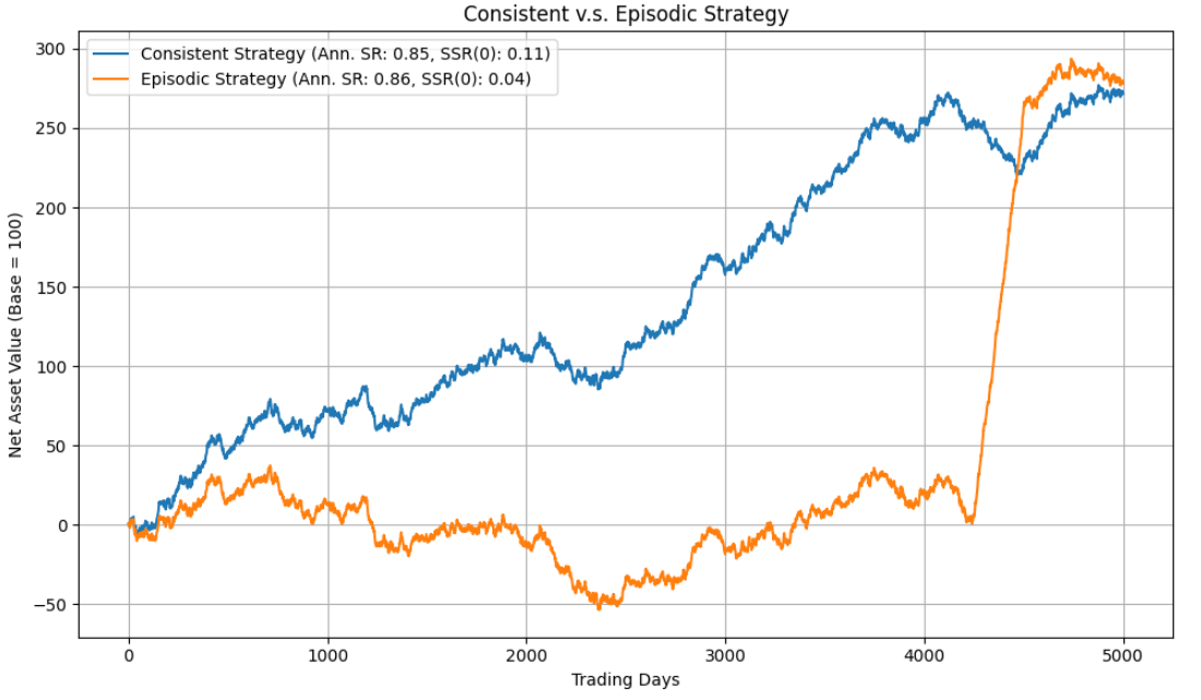
On Figure 8, the episodic strategy can be considered as a “crisis alpha” strategy while the consistent strategy can be considered as a “structural alpha” strategy.

In this case, relying on the Sharpe Ratio alone would not allow to distinguish between these two strategies and would actually favor the episodic strategy that exhibits a slightly higher Sharpe Ratio.

On the contrary, the Sharpe Stability Ratio properly favors³² the consistent strategy that generates persistent alpha⁸.

Practical considerations

How to choose the rolling window length?

Traver and Rodriguez Dominguez⁸ notes that the rolling window length $w$ is intrinsically a smoothing decision, analogous to selecting a bandwidth in nonparametric estimation: shorter windows produce noisy, high‑variance Sharpe estimates, whereas longer windows yield smoother but more “averaged‑out” dynamics⁸.

Thus, there is no universally applicable rolling window length.

That being said, standard rolling window sizes typically used in the litterature are the following:

• 252 days³³, for daily returns
• 52 weeks³⁴, for weekly returns
• 12 months³³, 36 months³⁵ or 60 months³³, for monthly returns

How to choose the benchmark Sharpe Ratio $SR_0$?

The benchmark Sharpe Ratio that appears in the Sharpe Stability Ratio formula plays a similar role to that of the benchmark Sharpe Ratio that appears in the Probabilistic Sharpe Ratio formula.

Nevertheless, the Sharpe Stability Ratio is somewhat unstable near the benchmark boundary⁸, which leads Traver and Rodriguez Dominguez⁸ to recommend using $SR_0 = 0$ as a base benchmark in empirical applications⁸.

Implementation in Portfolio Optimizer

The Portfolio Optimizer Web API allows to compute both the Sharpe Stability Ratio and the normalized Sharpe Stability Ratio as described in this blog post, c.f. the documentation.

Examples of usage

The Sharpe Stability Ratio v.s. the Sharpe Ratio

In the previous section, it has been empirically shown that the Sharpe Stability Ratio is complementary to the Sharpe Ratio, c.f. for example Figure 7 and Figure 8.

To illustrate the extent of that difference on real-world strategies with pronounced non-normality, serial dependence and regime-switching behavior⁸, Figure 9 plots the Sharpe Ratio v.s. the Sharpe Stability Ratio of the same 17 Barclay Hedge Fund Indices as used in Traver and Rodriguez Dominguez⁸ over the period January 1997 - December 2025.

As a side note, Figure 9 is the same as Figure 8 in Traver and Rodriguez Dominguez⁸, but independently reproduced using the Portfolio Optimizer Web API³⁶.

Figure 9. Sharpe Ratio v.s. Sharpe Stability Ratio, 17 Barclay Hedge Fund Indices, January 1997 - December 2025.

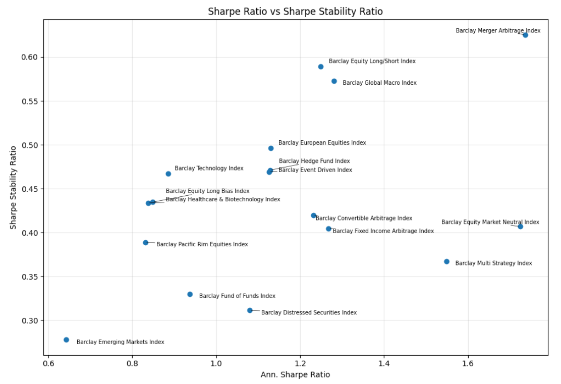
Figure 9 empirically shows again that there is not a one-to-one relationship between the Sharpe Ratio and the Sharpe Stability Ratio.

Thus, there is potentially an informational advantage in using the latter instead of the former!

The Sharpe Stability Ratio v.s. the Ulcer Performance Index

Martin⁹’s Ulcer Performance Index (UPI) - discussed elsewhere on this blog - is a prominent alternative³⁷ to the Sharpe Ratio, even though it does not fit within the mean-variance framework.

The Ulcer Performance Index replaces the standard deviation by the Ulcer Index (UI) as the risk measure, which makes it more directly comparable to the Sharpe Stability Ratio than the Sharpe Ratio because the Ulcer Index takes into account the temporal aspect of an investment returns.

In order to compare those two measures:

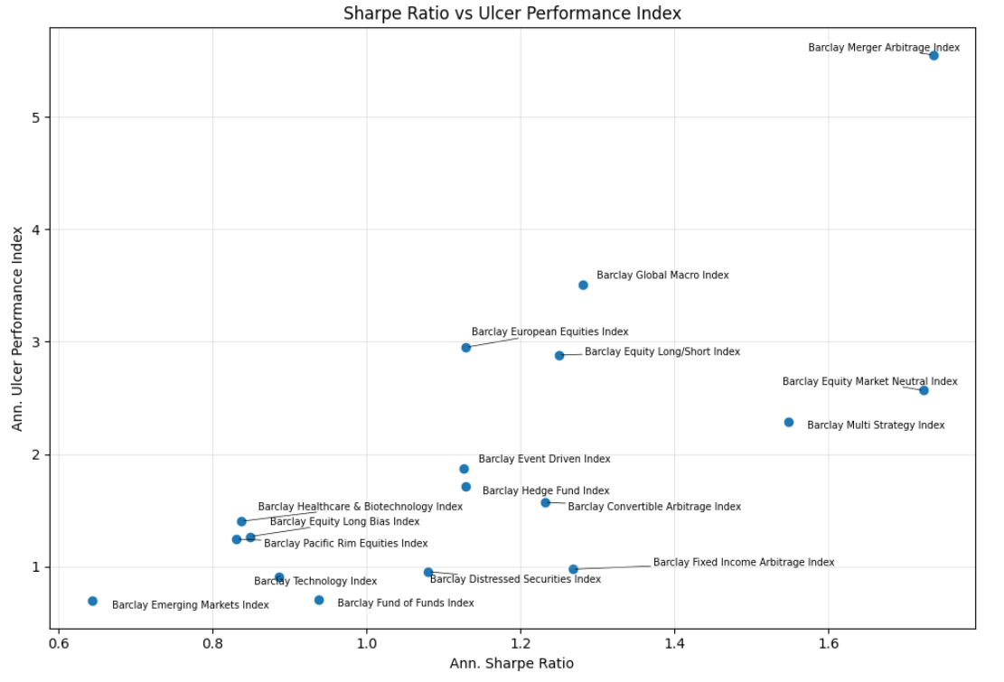
• Figure 10 plots the Sharpe Ratio v.s. the Ulcer Performance Index of the same 17 Barclay Hedge Fund Indices and over the same period as in the previous subsection.

  

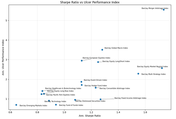
  Figure 10. Sharpe Ratio v.s. Ulcer Performance Index, 17 Barclay Hedge Fund Indices, January 1997 - December 2025.

  Figure 10 appears similar to Figure 9, which confirms that the Ulcer Performance Index also captures a different dimension of performance evaluation⁸ than the Sharpe Ratio.

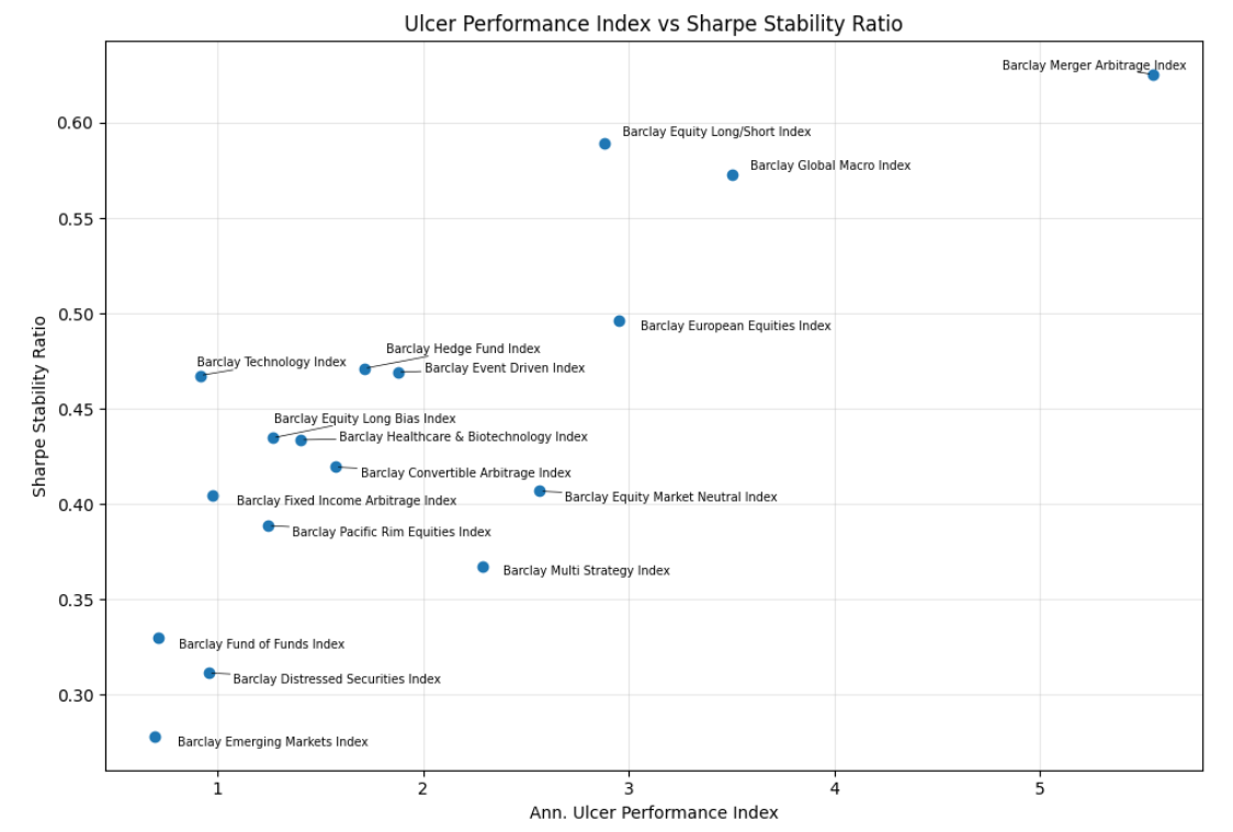
• Figure 11 plots the Ulcer Performance Index v.s. the Sharpe Stability Ratio of the same 17 Barclay Hedge Fund Indices and over the same period as in the previous subsection.

  

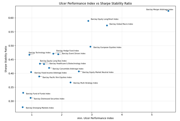
  Figure 11. Ulcer Performance Index v.s. Sharpe Stability Ratio, 17 Barclay Hedge Fund Indices, January 1997 - December 2025.

  The points displayed on Figure 11 are much closer to a straight line than in Figure 9 or in Figure 10, which highlights that the Ulcer Performance Index and the Sharpe Stability Ratio are close cousins.

  Not extremely close ones, though, because the correlation between these points is “only” of about 80%.

  In other words, people relying on the Ulcer Performance Index for risk-adjusted performance measurement might still find the Sharpe Stability Ratio to be an interesting addition to their arsenal!

The Sharpe Stability Ratio as a portfolio optimization objective

Following the same logic and for mostly the same reasons as in Bailey and de Prado⁷, it seems natural to extend [the Sharpe Stability Ratio] to a portfolio optimization or capital allocation context: rather than a mean-variance frontier of portfolio returns on capital, we will build a mean-variance frontier of portfolio [mean rolling] returns on risk⁷.

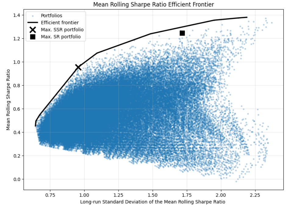
Figure 12 illustrates the idea of a Mean Rolling Sharpe Ratio Efficient Frontier, defined as the set of portfolios that deliver the highest expected mean rolling excess return on risk (as expressed by their mean rolling Sharpe Ratios) subject to the level of uncertainty surrounding those portfolios’ mean rolling excess return on risk (the long-run standard deviation of the mean rolling Sharpe Ratios).

Figure 12. Mean Rolling Sharpe Ratio Efficient Frontier, 10 multi-asset class ETFs, December 2006 - August 2023.

On Figure 12:

• Each blue point represents a portfolio within a universe of 10 ETFs representative of misc. asset classes³⁸, with each its mean rolling Sharpe Ratio and its long-run standard deviation of that mean rolling Sharpe Ratio
• The black line represents the Mean Rolling Sharpe Ratio Efficient Frontier, which is the set of portfolios whose mean rolling Sharpe Ratio is maximal for a given level of the long-run standard deviation of that mean rolling Sharpe Ratio
• The black cross represents the maximum Sharpe Stability Ratio portfolio, which plays a similar role on the Mean Rolling Sharpe Ratio Efficient Frontier than the maximum Sharpe Ratio portfolio on the usual mean-variance efficient frontier
• The black square represents the usual maximum Sharpe Ratio portfolio, for reference

It is interesting to note that the maximum Sharpe Stability Ratio portfolio and the maximum Sharpe Ratio portfolio seem pretty far appart in terms of their long-run standard deviation of their mean rolling Sharpe Ratio.

Do their holdings differ that much though?

Figure 13 answers that question.

Figure 13. Maximum Sharpe Stability Ratio v.s. maximum Sharpe Ratio portfolio holdings, 10 multi-asset class ETFs, December 2006 - August 2023.

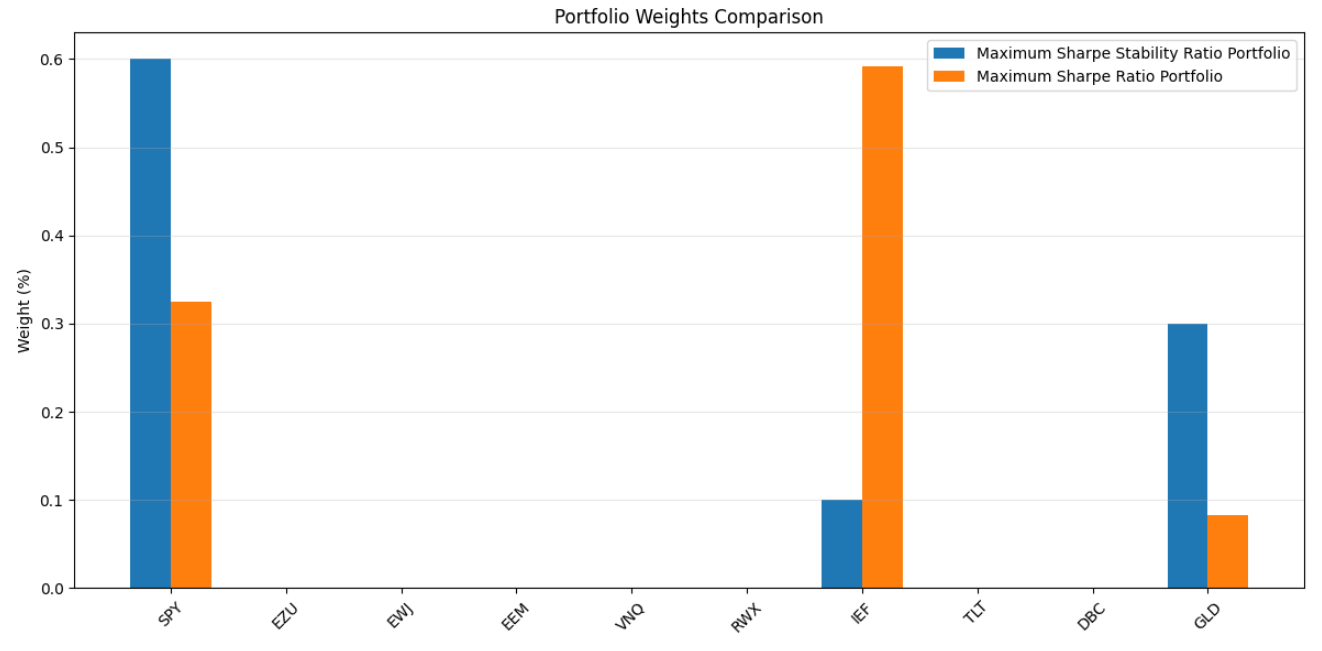
From Figure 13, these two portfolios share the same holdings³⁹ - U.S. stocks (SPY ETF), intermediate U.S. Treasuries (IEF ETF) and Gold (GLD ETF) - but with very different loadings, which is explained by their different opjectives:

• The maximum Sharpe Stability Ratio portfolio seeks to maximize its mean rolling Sharpe Ratio stability by diversifying its massive U.S. stocks exposure (60%) with intermediate U.S. Treasuries (10%) and Gold (30%)
• The maximum Sharpe Ratio portfolio seeks to maximize its point-in-time Sharpe Ratio by diversifying its massive intermediate U.S. Treasuries exposure (60%) with Gold (10%) and U.S. stocks (30%)

These nearly opposite loadings naturally lead to very different performances over time, depicted in Figure 14:

Figure 14. Maximum Sharpe Stability Ratio v.s. maximum Sharpe Ratio portfolio evolution, 10 multi-asset class ETFs, December 2006 - August 2023.

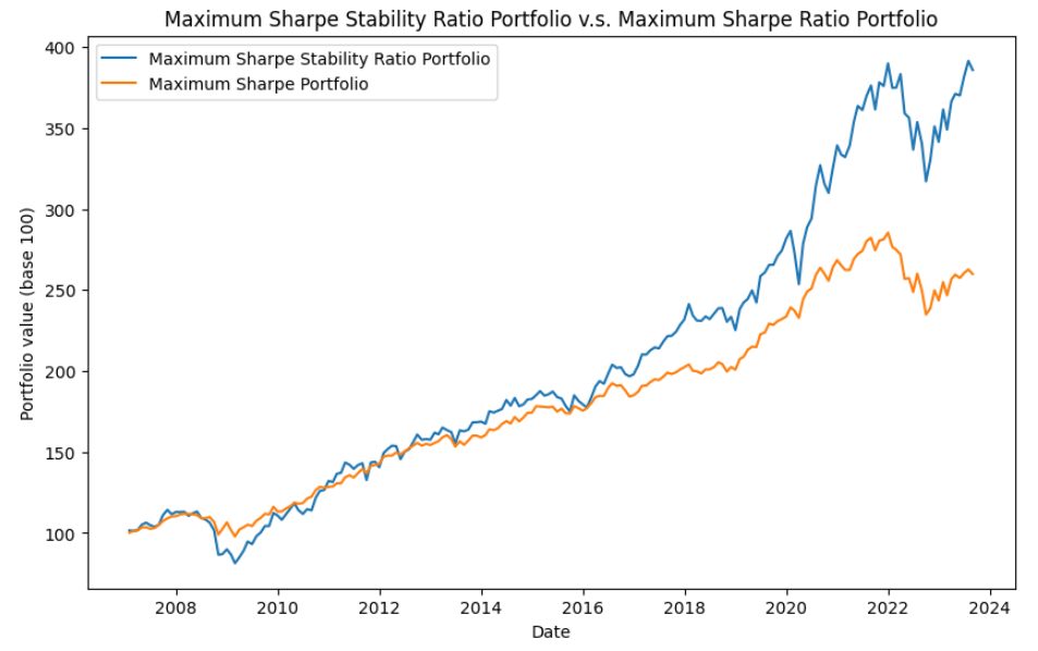
Additional figures below.

Portfolio	CAGR	Ann. Sharpe Ratio (0)	Sharpe Stability Ratio (0)	Maximum Drawdown
Maximum Sharpe Stability Ratio	8.44%	0.78	1	29%
Maximum Sharpe Ratio	5.90%	0.90	0.74	18%

Conclusion

This blog post detailled the Sharpe Stability Ratio, a statistically grounded method to incorporate temporal stability into performance evaluation by quantifying how much of a strategy’s Sharpe Ratio reflects persistent performance versus concentrated episodic strength⁸.

I hope you will find many applications for it in your trading!

While waiting to discover other performance measures, feel free to connect with me on LinkedIn or follow me on Twitter.

Notes:

• A big thanks to Mr Traver and Mr Rodriguez Dominguez who kindly provided me their implementation of the Sharpe Stability Ratio for comparison with my own.

–

1. See Sharpe, W., 1966, Mutual Fund Performance, Journal of Business, Vol. 39, No. 1, pp. 119–138. ↩ ↩²

2. C.f. de Prado et al.⁶, Sharpe ratios are used to report actual and backtested performance; identify new investment factors; rank, hire and fire portfolio managers; filter investment strategies (e.g., in due diligence questionnaires); define targets and constraints in portfolio optimization programs, etc³. ↩

3. See Lo, Andrew W. 2002. The Statistics of Sharpe Ratios. Financial Analysts Journal 58 (4): 36–52. ↩ ↩² ↩³

4. See Opdyke, J.D., Comparing Sharpe ratios: So where are the p-values?. J Asset Manag 8, 308–336 (2007). ↩ ↩²

5. At the date of publication of this blog post. ↩

6. See Marcos Lopez de Prado, Alexander Lipton, Vincent Zoonekynd, Sharpe Ratio Inference: A New Standard for Decision Making and Reporting, The Journal of Portfolio Management April 2026, 52 (6) 6-50. ↩ ↩² ↩³ ↩⁴ ↩⁵ ↩⁶ ↩⁷ ↩⁸ ↩⁹ ↩¹⁰ ↩¹¹ ↩¹² ↩¹³ ↩¹⁴ ↩¹⁵ ↩¹⁶ ↩¹⁷ ↩¹⁸

7. See Bailey, David H. and Lopez de Prado, Marcos, The Sharpe Ratio Efficient Frontier (April 1, 2012). Journal of Risk, Vol. 15, No. 2, Winter 2012/13. ↩ ↩² ↩³ ↩⁴ ↩⁵

8. See Bajo Traver, Mario and Rodriguez Dominguez, Alejandro, The Sharpe Stability Ratio: Temporal Consistency of Risk-Adjusted Performance. ↩ ↩² ↩³ ↩⁴ ↩⁵ ↩⁶ ↩⁷ ↩⁸ ↩⁹ ↩¹⁰ ↩¹¹ ↩¹² ↩¹³ ↩¹⁴ ↩¹⁵ ↩¹⁶ ↩¹⁷ ↩¹⁸ ↩¹⁹ ↩²⁰ ↩²¹ ↩²² ↩²³ ↩²⁴ ↩²⁵ ↩²⁶ ↩²⁷ ↩²⁸ ↩²⁹ ↩³⁰ ↩³¹ ↩³² ↩³³ ↩³⁴

9. See Martin, P. G. and B. B. McCann (1989). The Investor’s Guide to Fidelity Funds. Wiley. ↩ ↩²

10. As noted in Traver and Rodriguez Dominguez⁸, in empirical applications, $r_f$ is often replaced by its sample mean over the window without material effects, given the low variance of risk-free rates⁸. ↩

11. Depending on the authors, $\sigma_{r - r_f}^2$ is sometimes bias-corrected; in this blog post - and more generally on this website - bias correction is not used. ↩

12. See Lopez de Prado, Marcos, Sharpe Ratio Inference: A New Standard for Decision-Making and Reporting (Seminar Slides) (December 21, 2025). ↩

13. See Frank Schuhmacher, Martin Eling, A decision-theoretic foundation for reward-to-risk performance measures, Journal of Banking & Finance, Volume 36, Issue 7, 2012, Pages 2077-2082. ↩ ↩² ↩³ ↩⁴ ↩⁵

14. Emphasis on “most”, not “all”, which is also applicable to the Ulcer Performance Index, with Martin⁹ for example commenting that there is little difference between the [Ulcer Performance Index] and Traynor Index rankings of the funds⁹; nevertheless, that comment is not applicable when comparing strategies that seek to avoid major market downturns⁹. ↩

15. And, c.f. Schuhmacher and Elingby¹³, many distributions commonly used in finance satisfy the LS property¹³. ↩

16. Whatever the specific assumptions, the general idea is that the higher the non-normality/iid-ness of the excess return generating process, the higher the variance of its Sharpe Ratio. ↩

17. For the interested reader, the statistical inferential framework - much less practionner-friendly than the simple Probabilistic Sharpe Ratio formula - is detailled in a couple of previous blog posts (here and there). ↩

18. $SR_0$ is usually taken equal to 0 (no skill), 0.5 (annualized) or 1 (annualized). ↩ ↩²

19. To its author’s knowledge⁶, it is even the only one! ↩

20. See Newey, W. K., and K. D. West. A Simple, Positive Semi-definite, Heteroskedasticity and Autocorrelation Consistent Covariance Matrix. Econometrica. Vol. 55, No. 3, 1987, pp. 703-708. ↩ ↩²

21. While secondary to this blog post, but as an interesting side note, this choice is justified by the fact that the [first-order] Bartlett kernel is [typically] preferred in finite samples to the asymptotically optimal second-order kernel (the Quadratic Spectral (QS) kernel)⁴⁰; furthermore, Kolokotrones et al.⁴⁰ finds that no first-order kernel improves upon the Bartlett kernel⁴⁰. ↩

22. See Newey, W. K., and K. D. West. Automatic Lag Selection in Covariance Matrix Estimation. The Review of Economic Studies. Vol. 61, No. 4, 1994, pp. 631-653. ↩ ↩²

23. Rather than equivalent performances v.s. the benchmark. ↩

24. At least achievable over 10 years, and in all cases clearly more challenging than reaching a Sharpe Ratio greater than 1 over the same period of time. ↩

25. See Bernard, Carole and Boyle, Phelim P., Mr. Madoff’s Amazing Returns: An Analysis of the Split-Strike Conversion Strategy (May 14, 2009). Journal of Derivatives, Vol. 17, No. 1, 2009. ↩

26. Consistent with Traver and Rodriguez Dominguez⁸. ↩

27. Other variations are of course possible, like computing the Sharpe Stability Ratio of Fairfield Sentry over all subperiods of a given number of months and averaging them, etc. ↩

28. Other measures like the Deflated Sharpe Ratio (DSR)⁶ exist, but are better suited to other contexts; for example, when evaluating existing portfolios without proprietary backtesting (e.g., mutual funds, hedge fund indices, published ETFs), [the Deflated Sharpe Ratio] is less relevant — the evaluator performs no ex-ante selection over a large trial universe⁶. ↩

29. For reference, the 3 strategies share a Sharpe Ratio of 1.184 and Probabilistic Sharpe Ratios of 0.998 (0), 0.952 (0.5) and 0.673 (1.0). ↩

30. For reference, the Sharpe Stability Ratios (0) of the 3 strategies are 0.401 (A), 0.290 (B) and 0.321 (C). ↩

31. This one is inspired by Macrosynergy. ↩

32. General investors should also favor the consistent strategy, for many reasons: the single event around which the episodic strategy delivered nearly all its returns might never re-occur, 17 years is an extremely long time to wait for a strategy to deliver returns, etc. ↩

33. See Andrea Frazzini, Lasse Heje Pedersen, Betting against beta, Journal of Financial Economics, Volume 111, Issue 1, 2014, Pages 1-25. ↩ ↩² ↩³

34. See Xinyu Huang, Weihao Han, David Newton, Emmanouil Platanakis, Dimitrios Stafylas & Charles Sutcliffe (2023) The diversification benefits of cryptocurrency asset categories and estimation risk: pre and post Covid-19, The European Journal of Finance, 29:7, 800-825. ↩

35. See for example Burnside, Craig, et al. “Carry Trade: The Gains of Diversification.” Journal of the European Economic Association, vol. 6, no. 2/3, 2008, pp. 581–88. ↩

36. And using an independent source for Hedge Fund indices data. ↩

37. See Russ McBride, Alireza Dastan, Ulcer Index 2.6: A Better Risk Measure?, The Journal of Wealth Management Winter 2022, 25 (3) 59-71. ↩

38. U.S. stocks (SPY ETF), European stocks (EZU ETF), Japanese stocks (EWJ ETF), Emerging markets stocks (EEM ETF), U.S. REITs (VNQ ETF), International REITs (RWX ETF), U.S. 7-10 year Treasuries (IEF ETF), U.S. 20+ year Treasuries (TLT ETF), Commodities (DBC ETF), Gold (GLD ETF) ↩

39. Incidentaly, these are the ETFs that should compose a permanent portfolio… ↩

40. See Thomas Kolokotrones, James H. Stock, Christopher D. Walker, Is Newey–West optimal among first-order kernels?, Journal of Econometrics, Volume 240, Issue 2, 2024, 105399. ↩ ↩² ↩³