The Probabilistic Sharpe Ratio: Bias-Adjustment, Confidence Intervals, Hypothesis Testing and Minimum Track Record Length
The Sharpe ratio1 is one of the most commonly used measure of financial portfolio performance, but because it is deeply rooted in mean-variance theory, its usage with return distributions deviating from normality (e.g. hedge funds, cryptocurrencies) is frequently questioned2.
One solution to this issue is to switch to a probabilistic framework, under which the Sharpe ratio computed from a finite sample of observed returns is considered as a statistical estimator affected by error of an unobservable true Sharpe ratio, with the greater the non-normality of returns the greater the estimation error.
In this blog post inspired by the paper Comparing Sharpe ratios: So where are the p-values? from Opdyke3, I will summarize the main results of this probabilistic framework and I will use them to analyze the performances of a Bitcoin trading strategy recently published by the creator of the Bitcoin Stock-to-Flow model PlanB.
Notes:
- A Google sheet corresponding to this post is available here
Mathematical preliminaries
Let be:
- $r_1,…,r_T$ the observed returns of an asset/fund/portfolio/trading strategy/etc. over $T$ periods of time
- $\hat{\mu}$ the arithmetic average of these returns $\hat{\mu} = \frac{\sum_{t=1}^{T} r_t}{T}$
- $\hat{\sigma}$ the standard deviation4 of these returns $\hat{\sigma} = \sqrt{\frac{\sum_{t=1}^T (r_t - \overline{\mu})^2 }{T}}$
- $r_f$, the value of the risk free rate
Then, the Sharpe ratio $\widehat{SR}$ of the observed asset/fund/portfolio/trading strategy/etc. is defined as
\[\widehat{SR} = \frac{\hat{\mu} - r_f}{\hat{\sigma}}\]The usage of hats above emphases that $\hat{\mu}$, $\hat{\sigma}$ and $\widehat{SR}$ are quantities computed from the observed sample of returns $r_1,…,r_T$ while the true arithmetic average return $\mu$, the true standard deviation $\sigma$ and the true Sharpe ratio $ SR = \frac{\mu - r_f}{\sigma} $ are quantities associated with an unobservable return generating process.
It follows that $\hat{\mu}$, $\hat{\sigma}$ and $\widehat{SR}$ are statistical estimators of their true counterparts, subject to estimation error.
Extending the work of Mertens5 and Christie6, Opdyke3 derives the asymptotic statistical distribution for $\widehat{SR}$ under the general assumption of stationarity and ergodicity of returns
\[\widehat{SR} \overset{a}{\sim} N \left( SR, \frac{1 - \kappa SR + (\gamma - 1) \frac{SR^2}{4}}{T} \right)\], where $\kappa$ and $\gamma$ are respectively the true skewness and the true kurtosis of the unobservable return generating process.
This asymptotic statistical distribution provides a theoretical basis for making inference about the Sharpe ratio under the […] realistic conditions of time-varying conditional volatilities, serial correlation, and otherwise non-iid returns3, and Opdyke uses it to establish several properties of the Sharpe ratio estimator $\widehat{SR}$.
Confidence intervals for $\widehat{SR}$
The asymptotic statistical distribution for $\widehat{SR}$ enables to build three confidence intervals at a confidence level $100(1 - \alpha)$% for $\widehat{SR}$.
Using the notation $\widehat{SE(\widehat{SR})} = \sqrt{\frac{1 - \hat{\kappa} \widehat{SR} + (\hat{\gamma} - 1) \frac{\widehat{SR}^2}{4}}{T}}$ for the estimator of the standard error of $\widehat{SR}$, these are7:
- The two-sided confidence interval
- The lower one-sided confidence interval
- The upper one-sided confidence interval
, where the quantity $\hat{\kappa}$ (resp. $\hat{\gamma}$) is an estimator of $\kappa$ (resp. $\gamma$) computed from the observed sample of returns $r_1,…,r_T$ and $z_{1-\frac{\alpha}{2}}$ (resp. $z_{1-\alpha}$) is the $1−\frac{\alpha}{2}$ (resp. $1-\alpha$) critical value of the standard normal distribution.
Using one of the interpretations of confidence intervals, each of these confidence intervals represents values that are not statistically significantly different from $\widehat{SR}$ at a confidence level $100(1 - \alpha)%$.
It is interesting to note that while $\widehat{SR}$ depends only on
- The arithmetic average of the observed returns $\hat{\mu}$
- The standard deviation of the observed returns $\hat{\sigma}$
, the standard error of $\widehat{SR}$ depends on
- The arithmetic average of the observed returns $\hat{\mu}$
- The standard deviation of the observed returns $\hat{\sigma}$
- The skewness of the observed returns $\hat{\kappa}$
- The kurtosis of the observed returns $\hat{\gamma}$
- The number of observed returns8 $T$
Figure 1, taken from Bailey and de Prado9, illustrates how exactly the standard error of $\widehat{SR}$ is impacted by the true skewness and the true kurtosis in the case of a return generating process made of a mixture of two Gaussians with $SR$ equal to 1.
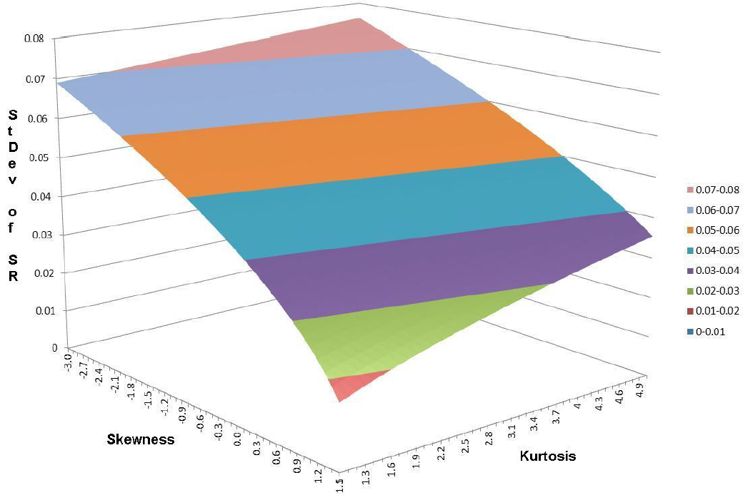
As they put it9:
although skewness and kurtosis does not affect the point estimate of $SR$, it greatly impacts its confidence bands, and consequently its statistical significance.
More on kurtosis does not affect the point estimate of $SR$ right away, though.
Small sample bias of $\widehat{SR}$
Opdyke3 provides the following bias adjustment formula for $\widehat{SR}$, valid for any return distribution
\[E \left[ \widehat{SR} \right] = SR \left( 1 + \frac{1}{4} \frac{\gamma - 1}{T} \right)\]Thus, while it is true that kurtosis does not affect the point estimate of $SR$, kurtosis do affect the unbiased point estimate of $SR$!
Hypothesis testing for $\widehat{SR}$
The asymptotic statistical distribution for $\widehat{SR}$ also enables to create statistical tests.
In the context of performance evaluation, a test of interest is to determine whether a given value of $\widehat{SR}$ is statistically significantly greater than a reference Sharpe ratio $c$, with typically:
- A reference Sharpe ratio of $c = 0$ reflecting excess returns relative to the risk free rate10
- A reference Sharpe ratio of $c = 1$ (annualized) reflecting excess returns relative to volatility
For this test:
- The exact statistical test to use is the one-sided right-tailed hypothesis test with significance level $\alpha$11
- The t-statistic3 is equal to
-
The critical value is $z_{1-\alpha}$, the $1-\alpha$ critical value of the standard normal distribution
-
The p-value is equal to
, where $\Phi$ is the cumulative distribution function of the standard normal distribution.
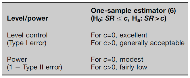
- Opdyke3 provides guidance on the type I and type II errors, reproduced in Figure 2 for convenience.
The Probabilistic Sharpe ratio $\widehat{PSR}$
To avoid referring to the statistical machinery of hypothesis testing, Bailey and de Prado9 introduced the Probabilistic Sharpe ratio $\widehat{PSR}(c)$, defined as the probability that the Sharpe ratio estimator $\widehat{SR}$ is greater than a reference Sharpe ratio $c$, which
takes [negative skewness and fat tails] into account and delivers a corrected, atemporal measure of performance expressed in terms of probability of skill
The Probabilistic Sharpe ratio is by definition equal to 1 minus the p-value of the hypothesis test from the previous section, so that12
\[\widehat{PSR}(c) = \Phi\left( \frac{\widehat{SR} - c}{ \sqrt{\frac{1 - \hat{\kappa} \widehat{SR} + (\hat{\gamma} - 1) \frac{\widehat{SR}^2}{4}}{T}} } \right )\]To be noted that the Probabilistic Sharpe ratio provides the same level of information as the p-value of this hypothesis test, so that using one or the other is a matter of personal preference.
The Minimum Track Record Length $\widehat{MinTRL}$
Because the value of the Probabilistic Sharpe ratio increases with the number of observed returns, which corresponds to the length of the track record in case of a fund or a trading strategy, Bailey and de Prado9 also introduced the Minimum Track Record Length $\widehat{MinTRL}(c)$, defined as the minimum number of observed returns required to ensure at a confidence level $100(1 - \alpha)$% that $\widehat{SR}$ is greater than a reference Sharpe ratio $c$.
The Minimum Track Record Length is equal to13
\[\widehat{MinTRL}(c) = \left( 1 - \hat{\kappa} \widehat{SR} + (\hat{\gamma} - 1) \frac{\widehat{SR}^2}{4} \right) \left( \frac{ z_{1-\alpha} }{\widehat{SR} - c} \right)^2\]Implementation in Portfolio Optimizer
In Portfolio Optimizer, the following endpoints are implemented:
/portfolios/analysis/mean-variance/sharpe-ratio/confidence-interval, to compute the various confidence intervals for the Sharpe ratio of a portfolio/portfolios/analysis/mean-variance/sharpe-ratio/probabilistic, to compute the Probabilistic Sharpe ratio of a portfolio
Examples of usage
Skillful hedge fund styles
I will first reproduce the results of Bailey and de Prado9 and perform an analysis of the HFRI Indices.
For this, I use the monthly indices levels over the period from the 31st December 1999 to the 30th May 201114 downloaded from the HFR website and compute the values $\widehat{SR}$, $\widehat{PSR}(0)$ and $\widehat{PSR}(\frac{0.5}{\sqrt12})$15.
The results are reported in Figure 3.
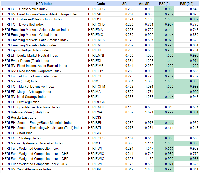
Compared to Bailey and de Prado9, data for three indices are missing16 plus the computed values for the other indices are slightly different17, but their two conclusions remain unaltered:
- Most of the HRF Indices exhibit a Probabilistic Sharpe ratio greater than 0 at a 95% confidence level
- Only 9 (+1, more on this below) HRF Indices exhibit a Probabilistic Sharpe ratio greater than 0.5 (annualized) at a 95% confidence level
One remark though.
The computations for the index HFRI Fund Weighted Composite Index - GBP completely differ between Bailey and de Prado and my reproduction, with for example a Sharpe ratio of $\approx 0.181$ v.s. $\approx 0.327$.
So, I strongly suspect that the underlying HFRIFWIG index data are not the same and that using Bailey and de Prado data, the Probabilistic Sharpe ratio of this index would not have been greater than 0.5 (annualized) at a 95% confidence level!
Analysis of a Bitcoin trading strategy
PlanB, the anonymous creator of the Bitcoin Stock-to-Flow model, recently released a trading strategy for Bitcoin.
This strategy, relying on the RSI technical indicator, is described in details PlanB’s article Quant Investing 10118 and produces the portfolio equity curve displayed in Figure 4, based on the reproduction of PlanB’s strategy by Andrea Meleri.
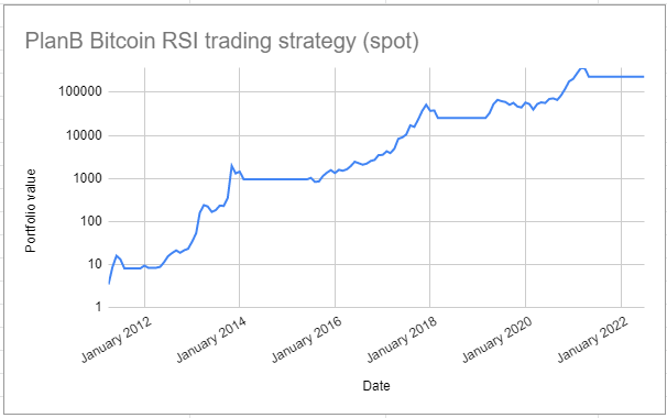
This strategy produces an annualized Sharpe ratio of $\approx 1$, but what about the statistical significance of this Sharpe ratio, especially since this strategy trades infrequently?
Thanks to the probabilistic framework presented in this blog post, it is possible to answer this question using for example the Probabilistic Sharpe ratio.
Indeed, as highlighted by Bailey and de Prado9:
It is not unusual to find strategies with irregular trading frequencies, such as weekly strategies that may not trade for a month. This poses a problem when computing an annualized Sharpe ratio, and there is no consensus as how skill should be measured in the context of irregular bets. Because PSR measures skill in probabilistic terms, it is invariant to calendar conventions.
I choose to compute the values $\widehat{PSR}(0)$, $\widehat{PSR}(\frac{0.5}{\sqrt 12})$, $\widehat{PSR}(\frac{0.75}{\sqrt 12})$ and $MinTRL(\frac{0.75}{\sqrt 12})$ at a confidence level of 95%, which are reported in Figure 5.

The values of $\widehat{PSR}(0)$ and $\widehat{PSR}(\frac{0.5}{\sqrt 12})$ support the hypothesis that this strategy exhibit some interesting performances, but the value of $\widehat{MinTRL}(\frac{0.75}{\sqrt 12})$ implies that around four years of additional returns19 are required in order to support the hypothesis that the real annualized Sharpe ratio of this strategy is greater than 0.75, which is still very far from 1!
In conclusion, this strategy definitely seems to be a good strategy, but due to its nature, there is not enough data yet to support the hypothesis that it is very good.
Conclusion
This is the end of this post, the first one in a series about the probabilistic framework for the Sharpe ratio.
In the second post of this series, I will present an additional result from Opdyke3 which enables to test whether two estimated Sharpe ratios are statistically different.
Meanwhile, and especially if you are a trading strategy developer, do not hesitate to do like QuantConnect and implement the Probabilistic Sharpe ratio as a performance evaluation metric, whether in-house or though a Web API call to Portfolio Optimizer!
–
-
See Sharpe, W., 1966, Mutual Fund Performance, Journal of Business, Vol. 39, No. 1, pp. 119–138. ↩
-
See Martin Eling, Frank Schuhmacher, Does the choice of performance measure influence the evaluation of hedge funds?, Journal of Banking & Finance, Volume 31, Issue 9, 2007, Pages 2632-2647. ↩
-
See Opdyke, J.D., Comparing Sharpe ratios: So where are the p-values?. J Asset Manag 8, 308–336 (2007). ↩ ↩2 ↩3 ↩4 ↩5 ↩6 ↩7
-
Following Christie20 and contrary to Opdyke3, I use $T$ in the computation of the standard deviation; for an extensive discussion about using $T$ v.s. $T-1$, see for example Carl R. Bacon21 or Sharpe himself22. ↩
-
See Mertens, E. (2002), Comments on the variance of IID estimator in Lo (2002, FAJ). ↩
-
See Christie, Steve, Is the Sharpe Ratio Useful in Asset Allocation? (May 2, 2005). Macquarie Applied Finance Centre Research Paper. ↩
-
To be consistent4, I use $T$ in the computation of the estimated standard error of the Sharpe ratio estimator $\widehat{SR}$. ↩
-
This justifies that Sharpe ratios are not comparable if calculated with a different number of return observations, c.f. Sharpe22. ↩
-
See Bailey, David H. and Lopez de Prado, Marcos, The Sharpe Ratio Efficient Frontier (April 1, 2012). Journal of Risk, Vol. 15, No. 2, Winter 2012/13. ↩ ↩2 ↩3 ↩4 ↩5 ↩6 ↩7
-
That is, reflecting skill of the portfolio manager. ↩
-
In practice, $\alpha$ is usually chosen equal to 0.05 to have a confidence level of 95%. ↩
-
To be consistent4, I use $T$ in the computation of the Probabilistic Sharpe ratio. ↩
-
Contrary to Bailey and de Prado9, the constant 1 does not appear in the formulation of the Minimum Track Record Length, because I used $T$ in the computation of the Probabilistic Sharpe ratio; this formulation is thus internally consistent. ↩
-
This is the closest period to the one used in Bailey and de Prado, which is 1st January 2000 to 1st May 20117. ↩
-
I took a value of the risk free rate equal to 0 for the different computations. ↩
-
HFRI EH: Priv/Regulation, HFRI EH: Short Bias and HFRI Russia-East Euro. ↩
-
Apart from the usage of $T$ v.s. $T-1$ in the definition of the Probabilistic Sharpe ratio12, the different computations are also sensitive to the formulas used for the kurtosis and the skewness. ↩
-
See Quant Investing 101. ↩
-
There are 136 monthly data points at the date of the publication of this blog post, and a $MinTRL$ value of $\approx 184$ means that $\approx 184 - 136 = \approx 48$ supplementary monthly data points are required in order to have $\widehat{PSR}(\frac{0.75}{\sqrt 12})$ greater than 95%. ↩
-
See Christie, Steve, Beware the Sharpe Ratio (January 2, 2007). ↩
-
See Carl R. Bacon, Practical Portfolio Performance Measurement and Attribution, 2nd Edition. ↩
-
See William F. Sharpe, The Sharpe Ratio, The Journal of Portfolio Management Fall 1994, 21 (1) 49-58. ↩ ↩2