The Probabilistic Sharpe Ratio: Hypothesis Testing and Minimum Track Record Length for the Difference of Sharpe Ratios
In the first post of this series about the Sharpe ratio considered as a statistical estimator, I introduced a probabilistic framework to answer the question
What is the probability that an estimated Sharpe ratio is statistically significantly greater than a reference Sharpe ratio?
In this second post, I will present additional results, described in the paper Comparing Sharpe ratios: So where are the p-values? from Opdyke1, to answer the slightly different question
What is the probability that an estimated Sharpe ratio is statistically significantly greater than another estimated Sharpe ratio?
As an example of application, I will show how to manage a portfolio of trading strategies characterized by uncertainty in their relative performances.
Notes:
- A Google sheet corresponding to this post is available here
Mathematical preliminaries
Let be:
- $r_{a,1},…,r_{a,T}$ and $r_{b,1},…,r_{b,T}$ the observed returns of two assets/funds/portfolios/trading strategies/etc. $a$ and $b$ over $T$ periods of time
- $\hat{\mu_a}$ and $\hat{\mu_b}$ the arithmetic averages of these returns $\hat{\mu_a} = \frac{\sum_{t=1}^{T} r_{a,t}}{T}$ and $\hat{\mu_b} = \frac{\sum_{t=1}^{T} r_{b,t}}{T}$
- $\hat{\sigma_a}$ and $\hat{\sigma_b}$ the standard deviations2 of these returns $\hat{\sigma_a} = \sqrt{\frac{\sum_{t=1}^T (r_{a,t} - \overline{\mu_a})^2 }{T}}$ and $\hat{\sigma_b} = \sqrt{\frac{\sum_{t=1}^T (r_{b,t} - \overline{\mu_b})^2 }{T}}$
- $r_f$, the value of the risk free rate
Then, the difference of the Sharpe ratios $\widehat{SR_{diff}} = \widehat{SR_a} - \widehat{SR_b}$ of the two observed assets/funds/portfolios/trading strategies/etc. is defined as
\[\widehat{SR_{diff}} = \frac{\hat{\mu_a} - r_f}{\hat{\sigma_a}} - \frac{\hat{\mu_b} - r_f}{\hat{\sigma_b}}\]The usage of hats above emphases that all the quantities $\hat{\mu_a}$, $\hat{\mu_b}$, $\hat{\sigma_a}$, $\hat{\sigma_b}$ and $\widehat{SR_{diff}}$ are computed from the two observed samples of returns $r_{a,1},…,r_{a,T}$ and $r_{b,1},…,r_{b,T}$ while the true arithmetic average returns $\mu_a$ and $\mu_b$, the true standard deviations $\sigma_a$ and $\sigma_b$ and the true difference of the Sharpe ratios $ SR_{diff} $ are quantities associated with two unobservable return generating processes.
In particular, it follows that $\widehat{SR_{diff}}$ is a statistical estimator of its true counterpart $ SR_{diff} $, subject to estimation error.
Opdyke1 derives the asymptotic statistical distribution of this estimator under the assumption of i.i.d. returns3
\[\widehat{SR_{diff}} \overset{a}{\sim} N \left( SR_{diff}, \frac{..._a + ..._b + ..._{a,b} }{T} \right)\], where:
- $…_a$ depends on $\kappa_a$ and $\gamma_a$, the true skewness and the true kurtosis of the unobservable return generating process associated to $a$
- $…_b$ depends on $\kappa_b$ and $\gamma_b$, the true skewness and the true kurtosis of the unobservable return generating process associated to $b$
- $…_{a,b}$ depends on the multivariate central moments of order $(1,1)$, $(1,2)$, $(2,1)$ and $(2,2)$ of the two unobservable return generating processes associated to $a$ and $b$
Hypothesis testing for $\widehat{SR_{diff}}$
The asymptotic statistical distribution of $\widehat{SR_{diff}}$ enables to build two-sample statistical tests.
In the context of performance comparison, a test of interest is usually to determine whether $\widehat{SR_a}$ is statistically significantly greater than $\widehat{SR_b}$.
For this test:
- The exact statistical test to use is the one-sided right-tailed hypothesis test with significance level $\alpha$4
which is equivalent, by definition, to
\[H_0: SR_a - SR_b \leq 0 \textrm{} \textrm{ v.s. } H_1: SR_a - SR_b > 0\]- The t-statistic is equal to
, with $\widehat{SE(\widehat{SR_{diff}})}$ the estimator of the standard error of $\widehat{SR_{diff}}$ equal to5
\[\widehat{SE(\widehat{SR_{diff}})} = \sqrt{\frac{\hat{..._a} + \hat{..._b} + \hat{..._{a,b}} }{T}}\]-
The critical value is $z_{1-\alpha}$, the $1-\alpha$ critical value of the standard normal distribution
-
The p-value is equal to
, where $\Phi$ is the cumulative distribution function of the standard normal distribution.
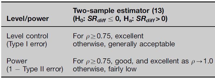
- Opdyke1 provides guidance on the type I and type II errors, reproduced in Figure 1 for convenience.
The generalized Probabilistic Sharpe ratio $\widehat{PSR}$
It is possible to generalize the Probabilistic Sharpe ratio $\widehat{PSR}$ of Bailey and de Prado6 to the two-sample statistical test above by defining the Probabilistic Sharpe ratio $\widehat{PSR_a}\left( SR_b \right) $ as the probability that the Sharpe ratio estimator $\widehat{SR_a}$ is greater than the Sharpe ratio estimator $\widehat{SR_b}$7.
The resulting Probabilistic Sharpe ratio is then by definition equal to 1 minus the p-value of the hypothesis test from the previous section, so that
\[\widehat{PSR_a}\left( SR_b \right) = \Phi\left( \frac{\widehat{SR_{diff}}}{ \widehat{SE(\widehat{SR_{diff}})} } \right )\]The generalized Minimum Track Record Length $\widehat{MinTRL}$
Similarly, it is possible to generalize the Minimum Track Record Length of Bailey and de Prado6 to the two-sample statistical test above by defining the Minimum Track Record Length $\widehat{MinTRL_a}(SR_b)$ as the minimum number of observed returns required to ensure at a confidence level $100(1 - \alpha)$% that $\widehat{SR_a}$ is greater than $\widehat{SR_b}$7.
The resulting Minimum Track Record Length is equal to
\[\widehat{MinTRL_a}(SR_b) = \left( \hat{..._a} + \hat{..._b} + \hat{..._{a,b}} \right) \left( \frac{ z_{1-\alpha} }{\widehat{SR_{diff}}} \right)^2\]Implementation in Portfolio Optimizer
In Portfolio Optimizer, the following endpoint is compatible with the two-sample statistical test above8:
/portfolios/analysis/mean-variance/sharpe-ratio/probabilistic, to compute the Probabilistic Sharpe ratio
Example of application - $\widehat{PSR}$-weighted portfolio of trading strategies
In their blog post Probabilistic Sharpe Ratio, the guys at QuantDare simulate the returns of two hypothetical trading strategies over 52 weeks and compare their Probabilistic Sharpe ratios $\widehat{PSR_1}(0)$ and $\widehat{PSR_2}(0)$ to select the best strategy to invest in for the next 5 years.
While this approach is certainly fine, I have two main issues with it:
- It relies on the standard Probabilistic Sharpe ratio, which is theoretically not designed to make comparisons between two estimated Sharpe ratios9
- It is binary, in that it aims to invest either fully in strategy 1 or fully in strategy 2
To solve these two issues, I propose to use the generalized Probabilistic Sharpe ratio defined above.
For this, I will first reproduce the results from QuantDare thanks to the Python notebook they published on GitHub.
Figure 2 describe the theoretical properties of the two simulated strategies10.
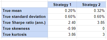
Figure 3 describe the estimated properties of the two simulated strategies, computed over the first 52 weeks of return data.
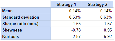
Comparing Figure 2 and Figure 3, it is clear that the estimated properties of these two strategies are completely different from their theoretical properties, with in particular $\widehat{SR_1} > \widehat{SR_2}$ while $SR_1 < SR_2$.
Hopefully, due to the non-normality of the observed returns, the standard Probabilistic Sharpe ratios $\widehat{PSR_1}(0)$ and $\widehat{PSR_2}(0)$ are such that $\widehat{PSR_1}(0) < 0.95 < \widehat{PSR_2}(0)$, c.f. Figure 4.
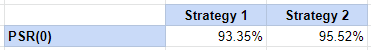
This shows that the standard Probabilistic Sharpe ratio appears to be able to select the true best strategy.
Nevertheless, if we compute the probability that the estimated Sharpe ratio $\widehat{SR_2}$ is greater than the estimated Sharpe ratio $\widehat{SR_1}$, we obtain $\widehat{PSR_2}(SR_1) \approx 48$%.
In other words, selecting strategy 2 v.s. strategy 111 as the true best strategy is actually akin to a flipping a coin!
Given this uncertainty, I propose to invest in both strategies proportionally to their respective generalized Probabilistic Sharpe ratio.
The exact rules of this strategy, that I will call the $PSR$-weighted strategy, are the following at the end of each week:
- Compute $\widehat{PSR_1}(SR_2)$ over an expanding window of returns12
- Invest $\widehat{PSR_1}(SR_2)$% of the current portfolio in strategy 1 and invest $(1 - \widehat{PSR_1}(SR_2))$% of the current portfolio in strategy 2
The associated equity curve for the next 5 years of simulated data is displayed in Figure 5, together with the equity curves of the two vanilla strategies.
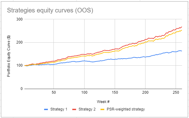
Figure 5 shows that the $PSR$-weighted strategy appears to be able to closely track the true best strategy, which makes it a sound strategy both in theory and in practice13.
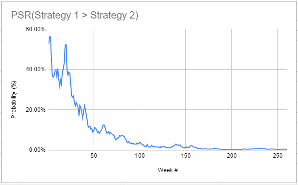
As a side note, this good tracking property comes from the quick convergence of $\widehat{PSR_1}(SR_2)$ to a negligible value, as illustrated in Figure 6.
Conclusion
The previous example concludes this second post.
In the third post of this series, I will present yet additional results, described in Bailey and de Prado14, to estimate the impact of multiple testing on the Sharpe ratio estimator.
–
-
See Opdyke, J.D., Comparing Sharpe ratios: So where are the p-values?. J Asset Manag 8, 308–336 (2007). ↩ ↩2 ↩3
-
Following Christie15 and contrary to Opdyke1, I use $T$ in the computation of the standard deviation; for an extensive discussion about using $T$ v.s. $T-1$, see for example Carl R. Bacon16 or Sharpe himself17. ↩
-
An open question raised in Opdyke1 is whether this derivation is valid under the general assumption of stationarity and ergodicity of returns. ↩
-
In practice, $\alpha$ is usually chosen equal to 0.05 to have a confidence level of 95%. ↩
-
To be consistent2, I use $T$ in the computation of the estimated standard error of the difference of the Sharpe ratios estimator $\widehat{SR_a} - \widehat{SR_b}$. ↩
-
See Bailey, David H. and Lopez de Prado, Marcos, The Sharpe Ratio Efficient Frontier (April 1, 2012). Journal of Risk, Vol. 15, No. 2, Winter 2012/13. ↩ ↩2
-
Mr. Opdyke was kind enough to provide me a reference Excel Sheet to validate the implementation in Portfolio Optimizer of this two-sample statistical test. While the results of Portfolio Optimizer differ from those of the Excel Sheet, the (small) differences are entirely explained by consistency reasons5. ↩
-
Indeed, the standard Probabilistic Sharpe ratio is based on a one-sample statistical test, c.f. the previous blog post. ↩
-
The risk-free rate is taken equal to 0 in all the computations. ↩
-
Or the reverse. ↩
-
The expanding window extends from the inception of the strategies 1 and 2 to the current week. ↩
-
Or at least in practice in a controlled simulation setting… ↩
-
See David H. Bailey and Marcos Lopez de Prado, The Deflated Sharpe Ratio: Correcting for Selection Bias, Backtest Overfitting, and Non-Normality, The Journal of Portfolio Management Special 40th Anniversary Issue 2014, 40 (5) 94-107. ↩
-
See Christie, Steve, Beware the Sharpe Ratio (January 2, 2007). ↩
-
See Carl R. Bacon, Practical Portfolio Performance Measurement and Attribution, 2nd Edition. ↩
-
See William F. Sharpe, The Sharpe Ratio, The Journal of Portfolio Management Fall 1994, 21 (1) 49-58. ↩