Tom Carlson’s Adaptive 60/40 Portfolio: Momentum-based Selection of Stock Diversifiers
Welcome to 2026, where bonds no longer diversify stocks, volatility remains elevated and inflation isn’t going anywhere1.
This is the dramatic, although factual, opening of Basis Points’s video Morgan Stanley’s asset allocation playbook for the next 5 years.
As a consequence, the 60/40 Portfolio - invested 60% in stocks and 40% in bonds - which for decades has stood as the institutional benchmark for ‘balanced’ portfolio allocation2 is showing signs of strain2 because bonds can not longer be counted on for downside protection during volatile equity markets3.
In this blog post, I propose to review an alternative to the 60/40 Portfolio recently4 proposed by Tom Carlson and called the Adaptive 60/40 Portfolio2.
After confirming that a regime change took place in 2022 by comparing the recent behaviour of bonds to their history, I will detail the construction rules of the Adaptive 60/40 Portfolio, analyze its performances and study a variation based on the Probabilistic Sharpe Ratio introduced in Bailey and de Prado5.
2022 - The year bonds changed
Figure 1, inspired by a LinkedIn post from Andreas Steiner, depicts two mean-variance efficient frontiers within a two-asset class universe made of:
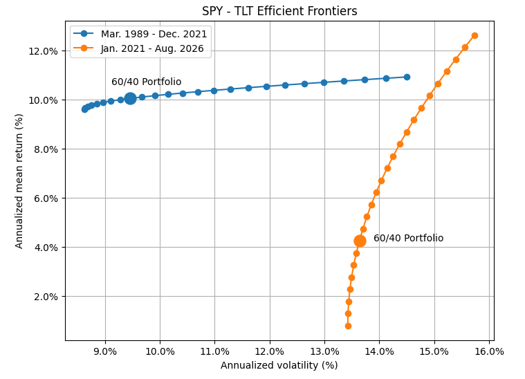
From Figure 1 and its underlying data, it is clear that the two periods 1989-2021 and 2022-2026 correspond to two different regimes, with the most recent period exhibiting:
- A huge increase in the correlation between stocks and bonds (from -0.12 to 0.57)
- A slight increase in stocks mean return (from 9.09% to 10.5%) and volatility (from 14.50% to 15.73%)
- A huge decrease in bonds mean return (from 7.23% to -0.64%) and a significant increase in their volatility (from 11.93% to 14.66%)
Figure 1 also confirms that the 60/40 Portfolio underwent marked changes8 in terms of risk-adjusted returns over these two periods, which explains the many reports about its death since 2022.
That being said, all portfolios actually underwent similar changes, so that there is nothing specific to the magic number duo 60/409.
The follow-up question - will this regime change last? - is harder to answer since it’s difficult to make predictions, especially about the future, but if history is any guide, it could last several years.
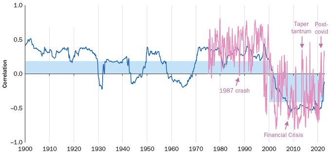
That prediction is supported by Figure 2, which shows that the positive correlation between stocks and bonds experienced since 2022 is not abnormal at all.
As Asness et al.10 puts it:
Even though this correlation was usually negative from 2000-2020, it was more often than not positive from 1900-2000. So a positive stock-bond correlation is hardly unprecedented; in fact, it’s been the historical norm.
As a consequence, while reports of [the 60/40 Portfolio] death are greatly exaggerated, that portfolio could use some fine-tuning to make it more compatible with the current regime.
The Adaptive 60/40 Portfolio
Rationale
The main observation from the previous section is that the traditional bond sleeve [of the 60/40 Portfolio] is showing signs of strain2 in the current market regime characterized by positively correlated stock and bond returns, hightened bond returns volatility and lowered bond returns.
In this new regime, the 40% intended to act as ballast during periods of market stress2 needs to be refined in two directions:
-
In terms of composition, incorporating alternative asset classes across both public and private markets is essential3
Indeed, since bonds are less reliable than in the (recent) past to diversify stock market exposure, other alternative investments need to be incorporated into the 40% defensive sleeve.
Beware of false diversifiers, though, for which returns can be explained by exposure to stock market risk10.
As Asness et al.10 puts it:
Too often [diversifiers] include stuff that has even more equity market risk than bonds – we’ve seen (among others) privates, buffer funds, and yes, even crypto.
In examples like these, investors trying to improve portfolio diversification end up making it worse.
-
In terms of dynamicity, it needs to be made adaptive
Here, Carlson11 highlights that most portfolios […] rely on static diversification11.
However, during periods of market panic, asset correlations tend to rise and fixed allocations can become vulnerable11.
For example, bonds, often seen as a hedge, have sometimes failed to protect capital during dislocations driven by inflation or policy shocks11.
Thus, the 40% defensive sleeve must be made adaptative, which serves multiple roles11:
- Macro Diversifier: Responds to shifting economic regimes
- Crisis Mitigator: Dynamically limits drawdowns
- Risk-Off Core: Generates positive expected return with lower volatility
- Anti-Correlation Sleeve: Low correlation to both equities and bonds, especially during systemic stress
Those two refinements are explained in very simple terms by Alexandre Ventelon, Morgan Stanley Wealth Management Australia Head of Investment Strategy and Solutions1:
So our recommendation has been with our clients, you need to diversify your diversifiers. You need to have a broader range. They will not all work at the same time.
In this context, Carlon’s2 Adaptive 60/40 Portfolio2 proposes to replace the static 40% bonds allocation of the 60/40 Portfolio by a dynamic 40% allocation into whichever defensive asset displays the strongest multi-period momentum among [three] liquid macro hedges2:
- Bonds, which are still useful as part of an overall portfolio, even with recently higher correlations10, because there’s little else out there that performs as consistently-well during recessions and related environments of falling growth10
- Gold, that responds positively to monetary instability and declining real rates11
- Broad commodities, that perform during stagflation or commodity supply shocks11
This [dynamic] multi-asset structure ensures that [the 40% defensive sleeve] adapts to different economic shocks rather than relying on a single hedge11.
Construction rules
In exact details, the Adaptive 60/40 Portfolio construction rules are the following.
At the end of each month:
- Invest 60% of the portfolio into U.S. stocks, represented by the SPY ETF
- Invest 40% of the portfolio into the best ranked defensive asset based on the equally weighted average of absolute returns over 1, 3, 6, and 12-month lookbacks among:
- Long-term U.S. Treasuries, represented by the TLT ETF
- Gold, represented by the GLD ETF
- Commodities, represented by the DBC ETF
From these construction rules, a couple of comments:
-
The Adaptive 60/40 Portfolio has a static 60% allocation to stocks
There is no adaptivity here.
-
The defensive sleeve of the Adaptive 60/40 Portfolio relies on a relative strength momentum framework2
This makes it adaptive to current market conditions, whatever they are, but such a framework does not prevent from investing into a diversifier with paltry returns10.
For this, an absolute momentum filter would be needed, which is not present in the vanilla version of the Adaptive 60/40 Portfolio.
As a side note, such a filter exists in another portfolio allocation framework proposed by Carlson11 called Defense First11.
The interested reader is refered to Moskowitz et al.12 and the subsequent litterature for more information about absolute and relative momentum.
Performances
Figure 3 compares the evolution of the Adaptive 60/40 Portfolio over the period13 February 1989 - August 2026 to that of:
- The 60/40 Portfolio
- The Non-adaptive 60/40 Portfolio, which is the static portfolio invested 60% in stocks, 13.3% in long-term U.S. Treasuries, 13.3% in gold and 13.3% in commodities14
- The Adaptive 60/40 Portfolio
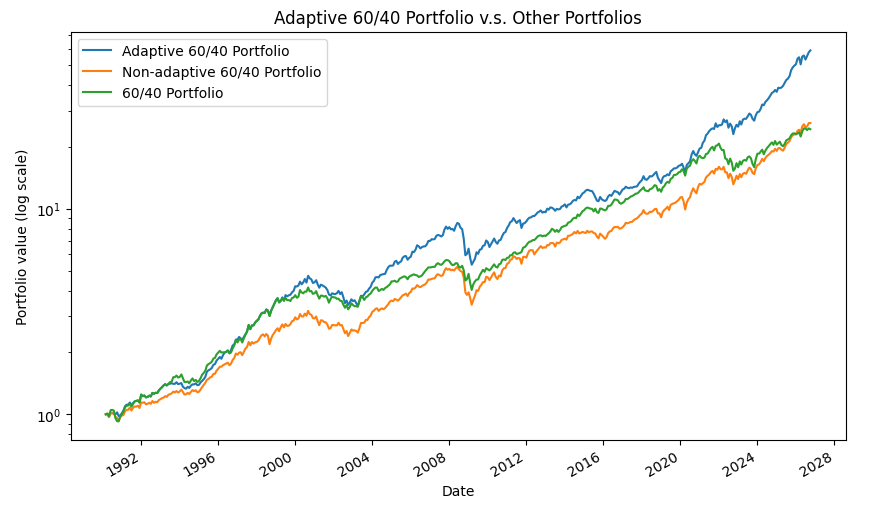
Figures below.
| Portfolio | CAGR | Ann. Standard Deviation | Ann. Sharpe Ratio (0) | Maximum Drawdown (monthly, end of month) |
|---|---|---|---|---|
| 60/40 Portfolio | 9.1% | 10.0% | 0.92 | 28.4% |
| Non-adaptive 60/40 Portfolio | 9.3% | 10.0% | 0.94 | 34.6% |
| Adaptive 60/40 Portfolio | 12.3% | 10.7% | 1.14 | 31.2% |
Those performances seem pretty compelling.
Neverthtless, as long-time readers of this blog might know, comparing a tactical(ish) asset allocation strategy to a static portfolio is difficult to justify…
For a fairer comparison, the Adaptive 60/40 Portfolio should rather be evaluated against its own true opportunity set15, which is the set of portfolios statisfying the following construction rules:
- Monthly rebalance at the end of each month
- Investment of 60% of the portfolio into the SPY ETF
- Investment of 40% of the portfolio into any combination of the TLT, GLD and DBC ETFs
The associated methodology - described elsewhere in this blog - leads to Figure 4, which contrasts the Sharpe Ratio of the Adaptive 60/40 Portfolio to that of 500,000 random portfolios representative of the true opportunity set mentioned above.
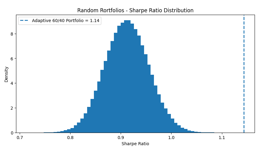
From Figure 4, the Sharpe Ratio of the Adaptive 60/40 Portfolio is much higher than nearly all the Sharpe Ratios achiveable within the considered true opportunity set, which is usually a sign of significant overfitting for a trading stragegy…
On the other hand, there is no apparent sign of overfitting in the construction rules of the Adaptive 60/40 Portfolio:
- The 60% allocation into U.S. stocks is inherited from the 60/40 Portfolio
- The 40% allocation into a defensive asset is a mathematical consequence16 of the 60% allocation into U.S. stocks
- The chosen defensive assets - long-term U.S. Treasuries, gold and commodities - all are standard stock diversifiers
- The tactical asset allocation strategy used in the defensive sleeve is backed by an abundant litterature on relative momentum across asset classes
So, ultimately, time will tell!
As a last remark, Carlson2 highlights that the correlation between the defensive sleeve of the Adaptive 60/40 Portfolio and U.S. stocks is nearly 0%17, which also makes it an interesting standalone stock diversifier.
Implementation
It is possible to follow live signals for Carlson’s Adaptive 60/40 Portfolio strategy on BestFolio (no affiliation).
Variation on the Adaptive 60/40 Portfolio
The tactical asset allocation strategy used in the defensive sleeve of the Adaptive 60/40 Portfolio is a monthly relative momentum strategy based on several momentum formation periods.
In details, at each monthly portfolio rebalancing date, multiple rankings are computed
| Asset | 1-month momentum | 3-month momentum | 6-month momentum | 12-month momentum |
|---|---|---|---|---|
| TLT ETF | $\text{TLT}_{1}$ | $\text{TLT}_{3}$ | $\text{TLT}_{6}$ | $\text{TLT}_{12}$ |
| GLD ETF | $\text{GLD}_{1}$ | $\text{GLD}_{3}$ | $\text{GLD}_{6}$ | $\text{GLD}_{12}$ |
| DBC ETF | $\text{DBC}_{1}$ | $\text{DBC}_{3}$ | $\text{DBC}_{6}$ | $\text{DBC}_{12}$ |
and are then converted into an aggregated ranking
| Asset | Aggregated momentum |
|---|---|
| TLT ETF | $\text{TLT}_{agg}$ |
| GLD ETF | $\text{GLD}_{agg}$ |
| DBC ETF | $\text{DBC}_{agg}$ |
in order to select the best overall defensive asset to hold for the next month.
Similar to Wouter et al.18, Carlson2 proposes to average the momentum observed over 1, 3, 6, and 12 months in order to span the optimal space and stabilize […] estimates18 so that formulas for the asset aggregated momentum signals are:
- $\text{TLT}_{agg} = \frac{1}{4} \left( \text{TLT}_{1} + \text{TLT}_{3} + \text{TLT}_{6} + \text{TLT}_{12} \right)$
- $\text{GLD}_{agg} = \frac{1}{4} \left( \text{GLD}_{1} + \text{GLD}_{3} + \text{GLD}_{6} + \text{GLD}_{12} \right)$
- $\text{DBC}_{agg} = \frac{1}{4} \left( \text{DBC}_{1} + \text{DBC}_{3} + \text{DBC}_{6} + \text{DBC}_{12} \right)$
I am personally not a big fan of such an aggregation mechanism for three reasons:
-
Equally averaging momentum signals (here, arithmetic returns) over different formation periods corresponds to an implicit weighting scheme
Typically, asset returns over a 12-month formation period are much higher in amplitude than asset returns over a 1-month formation period.
So, by equally averaging asset returns over different formation periods, much more weight is actually given to the longuest formation period v.s. the other formation periods.
This might be a desirable behavior, but if so, I would prefer it to be explicit.
-
Averaging momentum signals over different formation periods leads to uncontrolled cancellation of positive and negative asset returns
On top of the previous point, averaging asset returns over different formation periods makes positive and negative asset returns cancelling each other in a rather unpredictable and uncontrollable way.
This might also be a desirable behavior, but in that case, there must be ways to better control that behaviour.
-
Momentum signals have no built-in adaptability
The different lookback periods chosen in Carlson2 are quite common18 in the momentum litterature, but if - let’s say - momentum over a 6-month formation period did not work in the specific context of the Adaptive 60/40 Portfolio, it would have been excluded from its construction rules with a perfectly reasonable ex-post explanation.
That’s for the past, i.e., the backtest.
In addition, if at one point in time, momentum over - let’ say again - a 6-month formation period stops being predictive of relative asset returns over the next month, the Adaptive 60/40 Portfolio would not adapt19 to that evolution.
That’s for the future, i.e., live trading.
As an alternative aggregation mechanism, I would propose the following:
-
For each momentum lookback (1, 3, 6 and 12 months), transform the asset momentum signals into a cross-sectional percentile ranking20
-
Aggregate the resulting 4 cross-sectional percentile rankings into an overall percentile ranking through a statistical significance-based weighted average
Here, some comments are in order.
If - let’s say - the 6-month momentum signal has an history of being extremely predictive of next month’s relative asset returns v.s. the other lookbacks, the overall percentile ranking should reflect that in a way or another.
One possibility to achieve this objective is to compute the (normalized) average pairwise Probabilistic Sharpe Ratio of each $x$-month momentum signal - considered as a standalone trading strategy - against all the other $y$-month momentum signals with $x \ne y$.
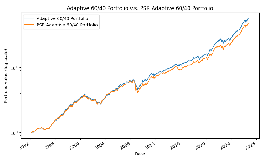
Figure 5 compares the evolution of the Adaptive 60/40 Portfolio over the period March 1992 - August 2026 to that of the resulting portfolio21, called the PSR Adaptive 60/40 Portfolio.
Figures below.
| Portfolio | CAGR | Ann. Standard Deviation | Ann. Sharpe Ratio (0) | Maximum Drawdown (monthly, end of month) |
|---|---|---|---|---|
| Adaptive 60/40 Portfolio | 12.4% | 10.7% | 1.15 | 31.2% |
| PSR Adaptive 60/40 Portfolio | 11.9% | 10.8% | 1.09 | 36.0% |
While there is a slight performance degradation in-sample22, I would be more confident in trading the PSR Adaptive 60/40 Portfolio out-of-sample.
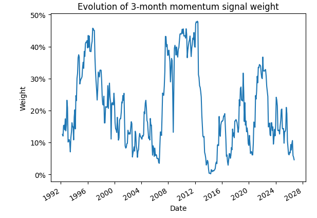
In any cases, Figure 6 confirms that the weights assigned to the different momentum lookbacks vary a lot, so that an evolutive weighting scheme is definitely something missing in the vanilla Adaptive 60/40 Portfolio.
As a side note, with this alternative aggregation mechanism, it is relatively harmeless to add other momentum formation periods - even apparently silly ones like 24 months - as well as to extend the universe of defensive assets.
One remaining caveat, though, is that there is still no absolute momentum filter in the defensive sleeve.
Perfect tinkering opportunity for the geeks out there :-) !
Conclusion
I leave the conclusion of this blog post to Carlson2:
Adaptive 60/40 is a simple framework for updating the defensive sleeve of balanced portfolios.
It’s transparent, easy to implement, and designed for allocators who need reliable tools — not complexity — to navigate evolving market regimes.
It’s not perfect, but it’s robust, repeatable, and built for the environments where static diversification breaks down.
To discover more tactical asset allocation strategies, feel free to connect with me on LinkedIn or follow me on Twitter.
–
-
See Morgan Stanley’s asset allocation playbook for the next 5 years, Basis Points by Equity Mates Media, 17 June, 2026 ↩ ↩2
-
See Tom Carlson, Adaptive 60/40: Rethinking the Defensive Sleeve, January 20, 2026. ↩ ↩2 ↩3 ↩4 ↩5 ↩6 ↩7 ↩8 ↩9 ↩10 ↩11 ↩12 ↩13
-
See Remi Olu-Pitan, Building portfolio resilience: why today’s approach needs to be different, Schroders, July 2025. ↩ ↩2
-
At the time of publication of this blog post. ↩
-
See Bailey, David H. and Lopez de Prado, Marcos, The Sharpe Ratio Efficient Frontier (April 1, 2012). Journal of Risk, Vol. 15, No. 2, Winter 2012/13. ↩
-
Extended with Fama and French data. ↩
-
Extended with the total returns associated to the U.S. 30-Year Treasury Constant Maturity Rates, c.f. a previous blog post for the associated methodology. ↩
-
An AI would have called these changes “structural”, but I did not use an AI to write this blog post. ↩
-
See Cliff Asness, Daniel Villalon, Antti Ilmanen, A Positive Stock-Bond Correlation Is a Terrible Reason to Add More Equity Risk to Your Portfolio, April 8, 2026 ↩ ↩2 ↩3 ↩4 ↩5 ↩6
-
See Carlson, Thomas, Defense First: A Multi-Asset Tactical Model for Adaptive Downside Protection (July 01, 2025). ↩ ↩2 ↩3 ↩4 ↩5 ↩6 ↩7 ↩8 ↩9 ↩10
-
See Tobias J. Moskowitz, Yao Hua Ooi, Lasse Heje Pedersen, Time series momentum, Journal of Financial Economics, Volume 104, Issue 2, 2012, Pages 228-250. ↩
-
Compared to Carlson2, this is an extended backtest made possible by the extension of the SPY and the TLT ETFs as already described in this blog post, and by the extension of the GLD and DBC ETFs thanks to the associated index data. ↩
-
In other words, the Non-adaptive 60/40 Portfolio corresponds to the non-tactical flavor of the Adaptive 60/40 Portfolio with 60% invested in stocks and 40% equally invested in all the defensive assets. ↩
-
See Roberto Stein, Not fooled by randomness: Using random portfolios to analyse investment funds, Investment Analysts Journal, 43:79, 1-15. ↩
-
Having 100% of a portfolio invested with 60% of that portfolio invested into an asset mathematically requires the remaining 40% of that portfolio to be invested into another asset. ↩
-
Exacty around 0.25% with the dataset used in this blog post. ↩
-
See Keller, Wouter J. and Butler, Adam and Kipnis, Ilya, Momentum and Markowitz: A Golden Combination (May 16, 2015). ↩ ↩2 ↩3
-
Pun intended. ↩
-
See Cakici, Nusret and Zaremba, Adam, Getting the Target Right in Return Prediction (April 20, 2026). ↩
-
I used a lookback of 24 months for computing the Probabilistic Sharpe Ratio; while this choice seems to be robust (i.e., using 18 months or 36 months does not materially affect the results), I would prefer to use 1 year of daily data in a real implementation. ↩
-
Which was predictable from Figure 4. ↩