Bootstrap Simulation with Portfolio Optimizer: Usage for Financial Planning

In statistics, a bootstrap method, also called bootstrapping, is a compute-intensive procedure that allows to estimate the distribution of a statistic through repeated resampling from a single observed sample of data¹.

Bootstrapping has several applications in quantitative finance, for example to test the robustness of a trading strategy, to compute a portfolio value at risk, etc.

In this post, I will describe the different bootstrap methods that are implemented in Portfolio Optimizer and I will illustrate the usage of a bootstrap method for financial planning.

Notes:

• A Jupyter notebook corresponding to this post is available on Binder -
• A good reference for bootstrap methods is the book Resampling Methods for Dependent Data from S. N. Lahiri².

Mathematical preliminaries

A bootstrap method typically follows the general three-step Monte Carlo algorithm described below³:

1. Bootstrap simulation step
   Generate $k \geq 1$ bootstrap samples $\hat{X}_{1,i}, …, \hat{X}^{*}_{n,i}, i=1..k$ through $k$ independent resamples with replacement from a sample of data $X_1, …, X_n$⁴⁵ observed from a population

2. Statistic computation step
   Compute a statistic of interest on the $k$ generated bootstrap samples

3. Statistic sampling distribution estimation step
   Approximate the sampling distribution of the statistic of interest thanks to the computed values of that statistic on the $k$ generated bootstrap samples

In the step 1 above, different resampling schemes lead to different bootstrap methods with different theoretical and practical properties.

In Portfolio Optimizer, three bootstrap methods are supported:

• The IID bootstrap
• The circular block bootstrap
• The stationary block bootstrap

Bootstrap method for non-dependent data - IID Bootstrap

The i.i.d. bootstrap method, originally introduced by Efron⁶, uses as resampling scheme a uniform sampling with replacement.

This bootstrap method is illustrated in Figure 1.

Figure 1. Example of i.i.d. bootstrap.

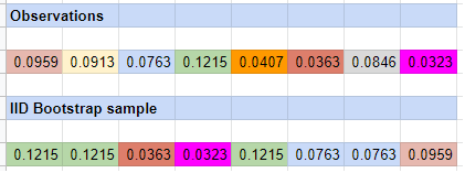
Theoretically, using the i.i.d. bootstrap method for inference requires that the observed sample of data consists of independent and identically distributed (i.i.d.) observations from a population⁷.

As a consequence, the i.i.d. bootstrap method is not appropriate in case of dependent data⁸, because resampling the individual observations $X_i, i=1..n$ independently of each other ignores any dependence structure (e.g. serial correlation) present in the observed sample of data.

This issue is illustrated in the context of U.S. equity returns by Capital Spectator in his blog post A Better Way To Run Bootstrap Return Tests: Block Resampling, from which Figure 2 and the associated comment is taken.

Figure 2. Example of i.i.d. bootstrap for the S&P 500 monthly returns. Source: Capital Spectator

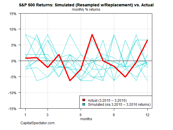
The problem is that the tendency for autocorrelation is severed [with the i.i.d. bootstrap]. In other words, the bootstrap sample is too random — the returns are independent from one another. In reality, that’s not an accurate description of market behavior.

Bootstrap methods for dependent data

Since the publication of the seminal paper of Efron, the i.i.d. bootstrap method has been extended to the case of dependent data by several authors, including for example Hall⁹, Carlstein¹⁰, Künsch¹¹ and Liu and Singh¹², and under several names (non-overlapping block bootstrap, moving block bootstrap…).

The common idea of most of these bootstrap methods for dependent data is to resample with replacement blocks of consecutive observations instead of single observations, which allows the dependence structure present within each block of the observed sample of data to be preserved.

Here again, different block resampling schemes lead to different bootstrap methods for dependent data, with different theoretical and practical properties.

Theoretically, using these block bootstrap methods for inference requires that the observed sample of data consists of weakly dependent stationary observations from a population².

To be noted, though, that it has been demonstrated that the moving block bootstrap method and the stationary block bootstrap method are both compatible with mild non stationarity¹³, which encompasses specific forms of serial dependence and heteroscedasticity.

Circular Block Bootstrap

The circular block bootstrap method, introduced by Politis and Romano¹⁴, uses as resampling scheme a uniform sampling with replacement of circular overlapping blocks of fixed length.

This bootstrap method is illustrated in Figure 3.

Figure 3. Example of circular block bootstrap.

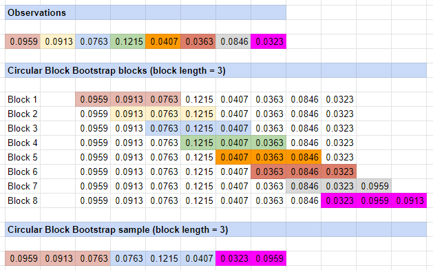
The circular block bootstrap method is an extension of the moving block bootstrap method of Künsch¹¹ and Liu and Singh¹² designed to fix the main shortcoming of the latter, which is that the observations at the beginning and at the end of the observed sample of data are undersampled in the bootstrap samples¹⁴.

The solution proposed by Politis and Romano visually consists in wrapping the observed sample of data around in a circle⁷.

Stationary Block Bootstrap

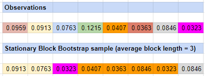
The stationary block bootstrap method, also introduced by Politis and Romano¹⁵, uses as resampling scheme a uniform sampling with replacement of circular overlapping blocks of random length.

Politis and Romano propose to use a geometric distribution with parameter $p \in ]0,1]$ for the blocks length, with $\frac{1}{p}$ corresponding to the average length of a block, in order to guarantee a theoretical property called conditional stationarity⁷, but any distribution can be used for the blocks length.

This bootstrap method is illustrated in Figure 4.

Figure 4. Example of stationary block bootstrap.

How to choose the block length?

It has been shown² both theoretically and empirically that the performances of block bootstrap methods depend significantly on the chosen block length¹⁶.

In order to choose an appropriate block length, it is possible to refer to:

• Theoretical results on the (asymptotic) optimal block length that have been established for example by Hall et al.¹⁷, who showed that the

  […] optimal block size depends significantly on context, being equal to $n^{\frac{1}{3}}$, $n^{\frac{1}{4}}$ and $n^{\frac{1}{5}}$ in the cases of variance or bias estimation, estimation of a one-sided distribution function, and estimation of a two-sided distribution function, respectively

• Practical results on the (finite sample) optimal block length that have been established for example by Politis and White¹⁸ and by Patton, Politis and White¹⁹, who introduced a data-driven procedure to compute an optimal block length based on the auto-correlation function of the observed sample of data.

In Portfolio Optimizer, the default block length (resp. average block length) has been chosen to be the same as in the R package tseries, that is, $ \lfloor 3.15 n^{\frac{1}{3}} \rfloor$ (resp. $3.15 n^{\frac{1}{3}}$), where $n$ is the size of the observed sample of data.

When the bootstrap method fails

Politis et al.²⁰ note that

Bootstrap methods can often achieve the goal of working in complex situations without imposing unrealistic or unverifiable assumptions about the data-generating mechanism, but like any statistical method, they cannot be applied without thought […] and [they] sometimes can fail.

Below are two examples of situations in which bootstrap methods can fail.

First, bootstrap methods are fundamentally dependent on the quality of the observed sample of data.

If this sample is not a reasonable representation of the underlying population (too small sample, biased sample, sample with an incorrect dependence structure…), the sampling distribution of any statistic of interest computed on the bootstrap samples will not be accurate.

Second, bootstrap methods are known to be inconsistent in some specific cases.

For example²¹, in the case of the i.i.d. bootstrap:

• The sampling distribution of the maximum of random variables converges to a random c.d.f.
• The sampling distribution of the mean of heavy tailed random variables converges to a random c.d.f.

Fortunately, it is usually possible to fix the inconsistency of a bootstrap method by generating bootstrap samples of $m < n$ observations²², but it is difficult in practice to determine a priori whether a given bootstrap method will be inconsistent for a given sample of observed data and a given statistic of interest.

As a side note, Portfolio Optimizer allows to generate bootstrap samples of any number of observations.

Example of usage - Financial planning

Since the seminal paper Determining Withdrawal Rates Using Historical Data of Bengen²³, financial planning using computer-based simulations, also known as Monte Carlo simulations, has become standard practice, c.f. for example the blog post The 3rd Generation of Financial Planning from Tolerisk or the sheer number of software providers offering goal based investing software solutions²⁴.

Although the future is impossible to predict, such simulations help to set realistic expectations about the potential performances of financial portfolios over long horizons and under real-life constraints²⁵ (e.g., periodic contributions or withdrawals, taxes, rising inflation rate, exposure to a sequence of return risk due to a bear market occurring at the wrong time…).

As an illustration of how Portfolio Optimizer could be integrated into a financial planning software, I will use the methodology of Anarkulova et al.²⁶ to simulate how a portfolio of U.S. stocks could be expected to behave over the next 30 years.

The exact methodology is the following:

1. Use the stationary block bootstrap method with an average block length of 120 months²⁷ to generate 10,000 bootstrap samples of 360 monthly returns²⁸ $\hat{R}_{1,i}, …, \hat{R}_{360,i}, i=1..10,000$ from the 1,428 U.S. stock market monthly returns²⁸ over the period January 1871 - December 1989 collected by Robert J. Shiller on his website
2. For each bootstrap sample $i=1..10,000$ and for each $h$-month horizon $h=1..360$, compute the projected cumulative wealth²⁹ at the $h$-month horizon $W_{h,i}$ associated to a fully invested buy and hold portfolio of U.S. stocks, with $W_{h,i}$ defined by $W_{h,i} = \prod_{t=1}^{h} \left( 1 + \hat{R}_{t,i} \right)$
3. For each $h$-month horizon $h=1..360$, compute the sampling distribution of $W_{h,i}$ over all the 10,000 bootstrap samples, and in particular compute
   • The median of this sampling distribution, which represents the (robust) expected projected cumulative wealth at the $h$-month horizon
   • The 2.5-th and 97.5-th percentiles of this sampling distribution, which represent the 95% bootstrap percentile confidence interval³ of the projected cumulative wealth at the $h$-month horizon
   • The 12.5-th and 87.5-th percentiles of this sampling distribution, which represent the 75% bootstrap percentile confidence interval³ of the projected cumulative wealth at the $h$-month horizon

More on why I considered U.S. stock returns only up to December 1989 later.

Step 1 is easily implemented thanks to the Portfolio Optimizer endpoint /assets/returns/simulation/bootstrap, while the ease of implementation of the remaining steps depends heavily on the environment (Google Sheets, C/C++, Python…)³⁰.

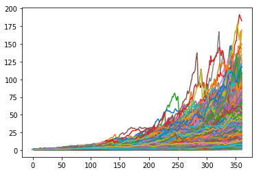
The results of step 2, that is, 10,000 projected cumulative wealth paths over 360 months, are illustrated in Figure 5.

Figure 5. Example of Monte Carlo simulation of asset returns (bootstrap) with Portfolio Optimizer.

For the sake of comparison, the results of an arbitrary Monte Carlo simulation performed by the Moneytree financial planning solution, taken from a presentation of Moneytree, are illustrated in Figure 6.

Figure 6. Example of Monte Carlo simulation with Moneytree. Source: Moneytree.

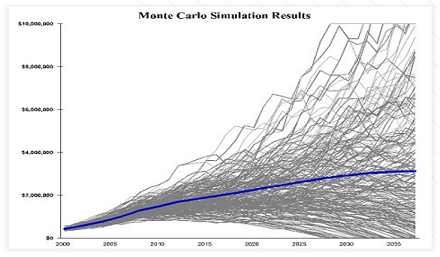
The similarities are striking…

The results of the step 3, that is, 360 medians and 360 2.5-th/12.5-th/87.5-th/97.5-th percentiles, are illustrated in Figure 7, together with the realized cumulative wealth over the period January 1990 - December 2019 which corresponds to the U.S. stock returns that I held out on purpose.

Figure 7. Example of Monte Carlo simulation of asset returns (bootstrap) with Portfolio Optimizer, and comparison with realized U.S. stock returns.

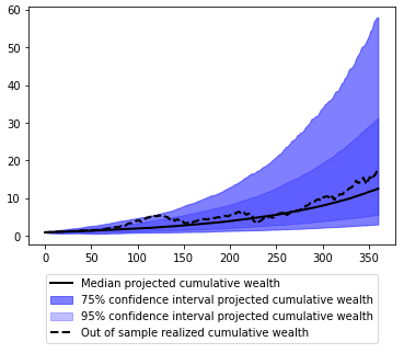
What is now striking is that the realized U.S. stock returns over the held-out period January 1990 - December 2019 are nearly always contained within the 95% bootstrap percentile confidence interval and are around three-quarter of the time contained within the 75% bootstrap percentile confidence interval…

While it seems that there might be black magic at work, this gives serious credibility to Monte Carlo simulations for financial planning!

Conclusion

Although this post only scratched the surface of the usage of bootstrap methods in portfolio management, I hope this feature of Portfolio Optimizer will be useful!

–

1. A strong assumption in any bootstrap method is that the observed sample of data is a reasonable representation of the underlying population, which somewhat guarantees that the distribution of the statistic over the resamples is a good approximation of the distribution of the statistic over the whole population. ↩

2. See Resampling Methods for Dependent Data, S. N. Lahiri, Springer Series in Statistics. ↩ ↩² ↩³

3. See B. Efron. R. Tibshirani. Bootstrap Methods for Standard Errors, Confidence Intervals, and Other Measures of Statistical Accuracy. Statist. Sci. 1 (1) 54 - 75, February, 1986. ↩ ↩² ↩³

4. The observations $X_1, …, X_n$ can be random variables or random vectors. ↩

5. In some bootstrap methods, like the parametric bootstrap, the observations $X_1, …, X_n$ are first used to build a statistical model of the population from which the bootstrap samples are then generated. ↩

6. See Efron, B. (1979), Bootstrap methods: Another look at the jackknife, The Annals of Statistics 7, 1-26. ↩

7. Hence the name of this bootstrap method. ↩ ↩² ↩³

8. There are different notions of dependent data in the literature, but the i.i.d. bootstrap is already not appropriate when the observed sample of data consists of $p$-dependent observations from a population, $p \geq 1$, c.f. Lahiri². ↩

9. See Hall, P. (1985), Resampling a coverage pattern, Stochastic Processes and Their Applications 20, 231-246. ↩

10. See Carlstein, E. (1986), The use of subseries methods for estimating the variance of a general statistic from a stationary time series, The Annals of Statistics 14, 1171-1179. ↩

11. See Künsch, H. R. (1989), The jackknife and the bootstrap for general stationary observations, The Annals of Statistics 17,1217-1261. ↩ ↩²

12. See Liu, R. Y. and Singh, K. (1992), Moving blocks jackknife and bootstrap capture weak dependence, in R. Lepage and L. Billard, eds, Exploring the Limits of the Bootstrap, Wiley, New York, pp. 225-248. ↩ ↩²

13. See Silvia Gonçalves, Dimitris Politis, Discussion: Bootstrap methods for dependent data: A review, Journal of the Korean Statistical Society, 2011, vol.40, no.4, pp. 383-386. ↩

14. See Politis, D. N. and Romano, J. P., A circular block resampling procedure for stationary data, in R. Lepage and L. Billard, eds, Exploring the Limits of Bootstrap, Wiley, New York, pp. 263-270. ↩ ↩²

15. See Politis, D. N. and Romano, J. P., The stationary bootstrap, Journal of the American Statistical Association 89, 1303-1313. ↩

16. Whether a fixed block length (moving block bootstrap, circular block bootstrap…) or an average block length (stationary bootstrap). ↩

17. See Hall, P., Horowitz, J. L. and Jing, B.-Y. (1995), On blocking rules for the bootstrap with dependent data, Biometrika 82, 561-574. ↩

18. See Dimitris N. Politis & Halbert White (2004) Automatic Block-Length Selection for the Dependent Bootstrap, Econometric Reviews, 23:1. ↩

19. See Andrew Patton , Dimitris N. Politis & Halbert White (2009) Correction to “Automatic Block-Length Selection for the Dependent Bootstrap” by D. Politis and H. White, Econometric Reviews, 28:4, 372-375. ↩

20. See Dimitris N. Politis, Joseph P. Romano, Michael Wolf, Subsampling, Springer Series in Statistics, 1999. ↩

21. See Fukuchi, Jun-ichiro, Bootstrapping extremes of random variables (1994). Retrospective Theses and Dissertations. 11256. ↩

22. This tweak is called the “$m$ out of $n$ bootstrap”²¹, and leads to the additional question of how to best choose the parameter $m$… ↩

23. See William P. Bengen, Determining Withdrawal Rates Using Historical Data, October 1994. ↩

24. Goal based investing software solutions, for example developed by MoneyGuidePro or WealthTrace, are typically using computer-based simulations due to the complexity of the underlying mathematical models. ↩

25. Such constraints are particularly important to take into account in the context of retirement planning, where the horizon is sometimes 50+ years. ↩

26. See Anarkulova, Aizhan and Cederburg, Scott and O’Doherty, Michael S., The Long-Horizon Returns of Stocks, Bonds, and Bills: Evidence from a Broad Sample of Developed Markets (November 15, 2021). ↩

27. Such an average block length has been shown²⁶ to capture the stylized facts of asset returns, including time-varying volatility and mean reversion. ↩

28. The monthly returns are total nominal returns (i.e., the consumer price index was forced to 1 in Shiller’s Excel sheet to explicitly discard inflation). ↩ ↩²

29. Starting from 1$. ↩

30. I used Python, c.f. the Jupyter notebook corresponding to this post available on Binder - . ↩