Random Portfolio Benchmarking: Simulation-based Performance Evaluation in Finance

As noted in Surz¹, the question “Is [a mutual fund’s]² performance good?” can only be answered relative to something¹, typically by comparing that fund to a benchmark like a financial index or to a peer group.

Unfortunately, these two methodologies are not without issues. For example, it is very difficult to create an index captur[ing] the essence of the people, process, and philosophy behind an investment product³ and peer groups have well-known biases¹ (classification bias, survivorship bias…).

In a series of papers (Surz³, Surz⁴, Surz¹…), Ronald J. Surz proposes an innovation that combines the better aspects of both [methodologies] while eliminating their undesirable properties³. This innovation consists in evaluating a fund against the fund manager’s true opportunity set⁵, defined as the set of all of the possible portfolios that the manager could have conceivably held following his unique investment process⁴.

In practice, the fund manager’s opportunity set is approximated by the simulation of thousands of random portfolios in the same universe of assets as the one of the fund manager and satisfying the same constraints (long-only, long-short…) and rules (portfolio rebalancing rules…) as those of the fund manager. Then, because these portfolios do not exhibit any particular skill⁶, they can be used as the control group to test [the] fund manager skill⁵, thus allowing to apply modern statistics to the problem of performance evaluation⁴.

In this blog post, I will describe how to generate random portfolios, detail Surz’s original methodology as well as some of its variations and illustrate the usage of random portfolios with a couple of examples like the creation of synthetic benchmarks or the evaluation and monitoring of trading strategies.

Mathematical preliminaries

Definition

Let be:

• $n$ the number of assets in a universe of assets
• $\mathcal{C} \subset \mathbb{R}^{n}$ a subset of $ \mathbb{R}^{n}$ representing the constraints imposed⁷ on a fund manager when investing in that universe of assets, for example:
  • Short sale constraints
  • Concentration constraints (assets, sectors, industries…)
  • Leverage constraints
  • Cardinality constraints (i.e., minimum or maximum number of assets constraints)
  • Portfolio volatility constraints
  • Portfolio tracking error constraints
  • …

Then, a (constrained) random portfolio in that universe of assets is a vector of portfolio weights $w \in \mathbb{R}^{n}$ generated at random over the set $\mathcal{C}$.

Generation at random v.s. generation uniformly at random

In the context of performance evaluation, as in Surz’s methodology, it is theoretically preferable that random portfolios are generated uniformly at random over the set $\mathcal{C}$, so as not to introduce any biases⁸ which would otherwise defeat the purpose of using these portfolios as an unbiased control group³.

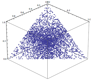
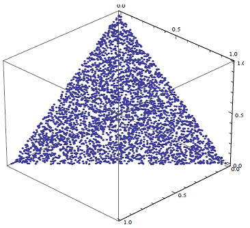
Figure 1 and Figure 2 illustrate the difference between random portfolios generated at random v.s. uniformly at random in the case of a three-asset universe subject to long-only and full investment constraints⁹:

• In Figure 1, the random portfolios are visibly concentrated in the middle of the standard 2-simplex in $\mathbb{R}^3$⁹ - these random portfolios are NOT generated uniformly at random
• In Figure 2, the random portfolios seem to be “well spread” over the standard 2-simplex in $\mathbb{R}^3$⁹ - these random portfolios are generated uniformly at random

Figure 1. Random portfolios not generated uniformly at random over a standard simplex, three-asset universe. Source: Shaw.

Figure 2. Random portfolios generated uniformly at random over a standard simplex, three-asset universe. Source: Shaw.

One important remark, though, is that real-life portfolios are usually binding on at least one of their constraints, so that generating random portfolios biased toward the boundary of the geometrical object associated to the constraints set $\mathcal{C}$ might not be a real problem in practice¹⁰.

Generation of random portfolios over the standard simplex

When the constraints imposed on a portfolio are 1) a full investment constraint and 2) a long-only constraint, the subset $C$ is then equal to

\[C = \{w \in \mathbb{R}^{n} \textrm{ s.t. } \sum_{i=1}^n w_i = 1, w_i \geq 0, i = 1..n\}\]

and the geometrical object associated to that subset is called¹¹ a standard simplex, already illustrated in Figure 1 and Figure 2 with $n = 3$.

Several algorithms exist to generate points uniformly at random over a standard simplex¹², among which:

• An algorithm based on differences of sorted uniform random variables
• An algorithm based on normalized unit exponential random variables

Generation of random portfolios over the restricted standard simplex

When the constraints imposed on a portfolio are 1) a full investment constraint, 2) a long-only constraint and 3) minimum/maximum asset weights constraints, the subset $C$ is then equal to

\[C = \{w \in \mathbb{R}^{n} \textrm{ s.t. } \sum_{i=1}^n w_i = 1, 1 \geq u_i \geq w_i \geq l_i \geq 0, i = 1..n\}\]

, where:

• $l_1, …, l_n$ represent minimum asset weights constraints
• $u_1, …, u_n$ represent maximum asset weights constraints

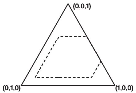
The geometrical object associated to that subset is a “restricted” standard simplex, as illustrated in Figure 3, with:

• $n = 3$
• $ 0.7 \geq w_1 \geq 0.1$
• $ 0.8 \geq w_2 \geq 0 $
• $ 0.6 \geq w_3 \geq 0.1 $

Figure 3. Example of restricted standard simplex, three-asset universe. Source: Piepel.

Generating points uniformly at random over a restricted standard simplex is much more complex than generating points uniformly at random over a standard simplex.

Hopefully, this problem has been studied at least since the 1990’s by people working in the statistical domain of the design of experiments, and an algorithm based on the conditional distribution method has been published¹³ in 2000.

Generation of random portfolios over a convex polytope

When the constraints imposed on a portfolio consist in generic linear constraints, the subset $C$ is then equal to

\[C = \{w \in \mathbb{R}^{n} \textrm{ s.t. } A_e w = b_e, A_i w \leq b_i \}\]

, where:

• $A_e \in \mathbb{R}^{n_e \times n}$ and $b_e \in \mathbb{R}^{n_e}$, $n_e \geq 1$, represent linear equality constraints
• $A_i \in \mathbb{R}^{n_i \times n}$ and $b_i \in \mathbb{R}^{n_i}$, $n_i \geq 1$, represent linear inequality constraints

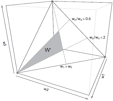
The geometrical object associated to that subset is called a convex polytope, illustrated in Figure 4, with:

• $n = 3$
• $\sum_{i=1}^n w_i = 1$
• $1 \geq w_i \geq 0, i = 1..n$
• $w_1 > w_2$
• $2w_3 > w_2 > 0.5w_3$

Figure 4. Example of standard simplex with additional linear inequality constraints, three-asset universe. Source: Tervonen et al.

As one can guess, generating points uniformly at random over a convex polytope is another level higher in terms of complexity, and while some algorithms exist to do so¹⁴, they are impractical in high dimension.

From the literature, what is possible to achieve instead is to generate points asymptotically uniformly at random, using Markov chain Monte Carlo (MCMC) algorithms like the Hit-And-Run algorithm¹⁵.

Generation of random portfolios over a generic constraint set

When the constraints imposed on a portfolio are generic, that is, quadratic (volatility or tracking error constraints) and/or non-convex (threshold constraints) and/or integer (maximum number of assets constraints, round lot constraints), the final boss has arrived.

With such constraints, the only reasonable¹⁶ approach in the literature seems to recast the problem of generating random points over the constraint set $C$ as a (penalized) optimization problem and use genetic algorithms to solve it¹⁰.

The underlying idea is to randomly¹⁷ minimize an objective function $f$ essentially made of penalties - the higher the distance of a point $w \in \mathbb{R}^{n}$ from the constraint set $C$, the higher the value of the objective function $f(w)$ -, so that at optimum, a random point satisfying all the constraints¹⁸ is found.

Of course, the points generated this way are not generated uniformly at random, but when the constraints are fully generic, that requirement should probably be dropped altogether as mentioned in Dawson and Young⁸.

Investment fund’s performance evaluation with random portfolios

Rationale

Evaluating the performance of an investment fund is actually a statistical hypothesis test in disguise¹⁹, in which:

• The null hypothesis is The investment fund’s exhibit no particular “performance” over the considered time period
• The test statistic is a quantitative measure of “performance” over the considered time period (e.g. annualized return, holding period return, risk-adjusted return…)
• The (empirical) distribution of the test statistic under the null hypothesis is computed from a sample made of either
  • One observation - the investment fund’s benchmark
  • A small number of observations - the investment fund’s peer group
  • Any desired number of observations - random portfolios generated from the investment fund’s universe of assets and obeying to the fund’s constraints and rules

From this perspective, using a benchmark, a peer group or random portfolios for performance evaluation is essentially a choice between sampling approaches¹.

Still, random portfolios represent a more rigorous approach to performance evaluation than the two other alternatives, for various reasons highlighted in different papers¹⁸¹⁰¹⁹ and summarized by Dawson⁸ as follows

A set of uniformly distributed, stochastically generated, portfolios that by construction incorporate no investment strategy, bias or skill form an effective control set for any portfolio measurement metric. This allows the true value of a strategy or model to be identified. They also provide a mechanism to differentiate between effects due to “market conditions” and effects due to either the management of a portfolio, or the constraints the management is obliged to work within.

Surz’s methodology

Using random portfolios to evaluate an investment fund’s performance over a considered time period is a two-step Monte Carlo simulation process²⁰:

1. Modeling step

   Identify the fund’s main characteristics.

2. Computational step

• Random portfolios simulation

  Generate random portfolios compatible with the identified fund’s main characteristics and simulate their evolution through the considered time period.

• Performance evaluation

  Determine the level of statistical significance of the fund’s performance over the considered time period using the previously simulated random portfolios.

Step 1 - Identifying the fund’s main characteristics

Dawson⁸ note that an investment strategy is essentially a set of constraints [and rules] that are carefully constructed to (hopefully) remove, in aggregate, poor performing regions of the solution space⁸. Thus, it is very important to identify as precisely as possible the main characteristics of the fund, even though this […] information is not always available, as only the manager knows [it] exactly¹⁹.

From a practical perspective, these characteristics need to be provided as²¹:

• A universe of $n$ assets modeling the fund’s universe of assets
• A constraint set $\mathcal{C} \subset \mathbb{R}^{n}$ modeling the fund’s constraints
• An ensemble of decision rules modeling²² the fund’s rebalancing rules

For examples of this step in different contexts, c.f. Kothari and Warner²³ and Surz²⁴.

Step 2a - Simulating random portfolios

Thanks to the previous step, it becomes possible to simulate thousands of random portfolios that the fund’s manager could have potentially held over the considered time period.

The only difficulty at this point is computational, due to the impact of the constraint set on the algorithmic machinery required to generate portfolio weights at random.

As a side note, and for a fair comparison [with the fund under analysis], transaction costs, as well as all other kinds of costs, must be considered¹⁰ when simulating random portfolios.

Step 2b - Evaluating the fund’s performance

The ranking of the fund’s performance against the performance of all the simulated random portfolios provides a direct measure of the statistical significance of that fund’s performance¹.

Indeed, under the null hypothesis that the investment fund’s exhibit no particular performance over the considered time period, the $p$-value of the statistical hypothesis test mentioned at the beginning of this section is defined as²⁵

\[p = \frac{n_x + 1}{N + 1}\]

, where:

• $n_x$ is the the number of random portfolios whose performance over the considered time period is as extreme or more extreme than that of the fund under evaluation
• $N$ is the number of simulated random portfolios

This idea is illustrated in Figure 5, which depicts:

• The distribution of the holding period return of 1000 random portfolios made of stocks belonging to the S&P 500 and subject to misc. turnover and cardinality constraints (solid line)
• The 95th percentile of that distribution (dashed line)

Figure 5. Distribution of the holding period return of random portfolios simulated from stocks belonging to the S&P 500, 2005 - 2010. Source: Stein.

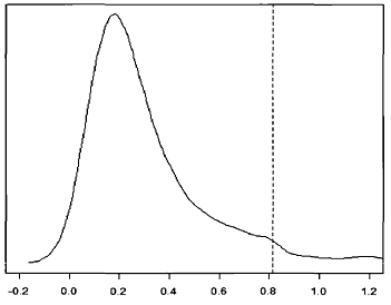
From this figure, if we were to evaluate the performances of a fund trading these securities and operating under constraints similar to those simulated, [it] would have to obtain a return equal of at least 80% during the 6 year period for the null of no particular performance to be rejected⁵ at a 95% confidence level.

Variations on Surz’s methodology

Burns¹⁰²⁵ and Lisi¹⁹ both extend Surz’s methodology from one time period to several time periods - which allows to consider the persistence of results over time¹⁹ - by describing different ways of combining individual $p$-values²⁶. As a by-product, Burns¹⁰²⁵ empirically demonstrates that Stouffer’s method²⁷ for combining $p$-values should be preferred to Fisher’s when evaluating a fund’s performance over multiple time periods.

Stein⁵ proposes to replace Surz’s methodology by testing whether the distribution of returns of the [fund under evaluation] is stochastically greater than that of [a] chosen percentile random fund using the Mann–Whitney U test.

Caveats

Surz¹ warns that there are many ways to implement a [Monte Carlo simulation] approach [with random portfolios], some better than others, and some worse¹.

In particular, Surz¹ argues that, when selecting a number of assets at random to satisfy portfolio cardinality constraints, it is required to use value-weighted sampling, so that the probability of choosing a given [asset] is proportionate to its outstanding capitalization¹. Otherwise, some macroeconomic [in]consistency¹ would be introduced by the Monte Carlo simulation process, which would ultimately bias the end results. This point is confirmed for both U.S. and global stocks in Arnott et al.²⁶, who show that random portfolios introduce, often unintentionally, value and small cap tilts²⁶. Nevertheless, other authors¹⁹ argue on the contrary that using equally-weighted sampling is more representative of the behavior of an “unskilled” manager, which is exactly what random portfolios are supposed to model!

More generally, random portfolios might have “unfair” characteristics v.s. the fund under evaluation (higher volatility, higher beta, lower turnover…), which must either be acknowledged or controlled for depending on the exact circumstances.

Implementations

Implementation in Portfolio Optimizer

Through the endpoint /portfolios/simulation/random, Portfolio Optimizer allows to:

• Generate the weights of a random portfolio subject to general linear inequality constraints

Through the endpoint /portfolios/simulation/evolution/random, Portfolio Optimizer allows to:

• Simulate the evolution of a random portfolio subject to general linear inequality constraints over a specified time period, with 3 different portfolio rebalancing strategies:
  • Buy and hold
  • Rebalancing toward the weights of the initial random portfolio
  • Rebalancing toward the weights of a new random portfolio

Implementations elsewhere

I am aware of two commercial implementations of random portfolios for performance evaluation as described in this blog post:

• Portfolio Probe, from Patrick Burns²⁸ of Burns Statistics
• PIPODs, from Ronald Surz²⁸ of PPCA Inc., which seems discontinued

Examples of usage

Hedge funds performance evaluation

The performances of hedge funds are notoriously difficult to evaluate due to the lack of both proper benchmarks and homogeneous peer groups²⁴.

Random portfolios offer a solution to this problem because they can reflect the unique specifications of each individual hedge fund²⁴.

More details can be found in Surz²⁴ or in Molyboga and Ahelec²⁹.

Investment strategy returns dispersion analysis

Kritzman and Page³⁰ uses random portfolios to compare the relative importance of different investment strategies (investment at global asset class level, at individual stock level, etc.) and concludes that³⁰

Contrary to perceived doctrine, dispersion around average performance arising from security selection is substantially greater than dispersion around average performance arising from all other investment choices. Moreover, asset allocation, widely considered the most important investment choice, produces the least dispersion; thus, from a normative perspective it is the least important investment choice.

Figure 6, which quantifies that dispersion around average performance, shows the extent to which a talented investor (top 25th or 5th percentile) could have improved upon average performance by engaging in various investment choices across a global universe. It also shows how far below average an unlucky investor (bottom 75th or 95th percentile) could have performed, depending on the choice of investment discretion³⁰.

Figure 6. 5th, 25th, 75th, and 95th percentile of the annualized difference from average performance of random portfolios simulated from misc. global asset classes, 1987-2001. Source: Kritzman and Page.

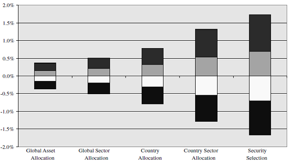
While this conclusion has been criticized³¹, the underlying methodology - returns dispersion analysis - provides valuable insight to investors in that it allows to understand the potential impact of [any] investment choice, irrespective of investment behavior³⁰.

For example, let’s suppose a French investor would like to passively invest in an MSCI World ETF, but is worried by both³²:

• The massive ~70% weight of the United States in that index
• The ridiculous ~3% weight of his home country in that index

Thus, this investor would rather like to invest in an MSCI World ETF “tilted” away from the United States and toward France, although he has no precise idea about how to implement such a tilt.

Here, returns dispersion analysis through random portfolios can help our investor understand the impact on performances of his proposed tactical deviation from the baseline investment strategy, at least historically³³.

For this, Figure 7 depicts the range of annualized returns achieved over the period 31 December 2008 - 29 December 2023 by 10000 random portfolios invested in the 23 countries of the MSCI World index when³⁴:

• The weights of the United States and France are made randomly varying between 0% and 100%
• The weights of all the other countries are kept constant v.s. their reference weights

Figure 7. Quartiles of the annualized returns of random portfolios from countries included in the MSCI World tilted away from the U.S. and toward France, 31 December 2008 - 29 December 2023.

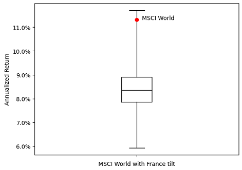
It is clear from from Figure 7 that deviating from the MSCI World index by under-weighting the United States and over-weighting France has been a relatively bad strategy over the considered period, with a median annualized return of ~8.30% compared to an annualized return of ~11.30% for the MSCI World³⁵!

Whether history will repeat itself remains to be seen, but thanks to this historical returns dispersion analysis, our investor is at least informed to take an educated decision re. his proposed investment strategy.

Synthetic benchmark construction

Stein⁵ proposes to use random portfolios in order to construct a “synthetic” benchmark, representative of all possible investment strategies within a given universe of assets and subject to a given set of constraints and rules.

In more details, Stein⁵ proposes to construct such a benchmark directly from the time series of returns of a [well chosen] single random portfolio⁵, which is typically the median¹ random portfolio w.r.t. a chosen performance measure.

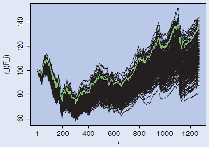
A similar idea is discussed in Lisi¹⁹, in which such a benchmark is this time constructed from the cross-sectional returns of the random portfolios.

Figure 8 illustrates Lisi’s methodology; on it, the green line represents a synthetic benchmark made of the 95th percentile³⁶ of the distribution of the random portfolios holding period returns at each time $t$

Figure 8. Time series of the 95th percentile of cross-sectional holding period returns of random portfolios. Source: Lisi.

The possibility to create synthetic benchmarks is particularly useful when evaluating the performances of tactical asset allocation (TAA) strategies, because their allocation might completely change from one period to another, making their comparison with a static benchmark - like a buy and hold portfolio or a 60/40 stock-bond portfolio - difficult to justify a priori.

For example, Figure 9 compares over the period 30th November 2006 - 31th January 2024³⁷:

• The Global Tactical Asset Allocation (GTTA)³⁸ strategy of Mebane Faber, which invests monthly - depending on the quantitative rules described in Faber³⁸ - within a five-asset universe made of:
  • U.S. Equities, represented by the SPY ETF
  • International Equities, represented by the EFA ETF
  • Intermediate-Term U.S. Treasury Bonds, represented by the IEF ETF
  • U.S. Real Estate, represented by the VNQ ETF
  • Global Commodities, represented by the DBC ETF
• An (equal-weighted) buy and hold portfolio within Faber’s five-asset universe, which is the benchmark of the GTTA strategy proposed in Faber³⁸
• A synthetic benchmark à la Lisi¹⁹ constructed from the median cross-sectional holding period returns of 25000 random portfolios simulated³⁹ within Faber’s five-asset universe

Figure 9. Global Tactical Asset Allocation (GTTA) strategy v.s. misc. benchmarks, 30th November 2006 - 31th January 2024.

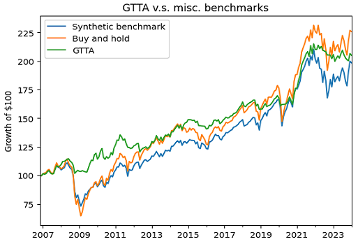
In Figure 9, the buy and portfolio and the synthetic benchmark both appears to behave quite similarly⁴⁰, but the synthetic benchmark should theoretically be preferred for performance comparison purposes because it better reflects the dynamics of the GTTA strategy (varying asset weights, varying exposure) while guaranteeing the complete absence of skill⁴¹.

Trading strategy evaluation

Random portfolios also find applications in evaluating (quantitative) trading strategies.

One of these applications, described in Dawson⁸, consists in evaluating the significance of an alpha signal through the comparison of two different samples of random portfolios:

It is […] very difficult to show conclusively the effect that a model, strategy […] has on the real investment process. […] The ideal solution would be to generate a set of portfolios, constrained in the same way as the portfolio(s) built with the theory or model under investigation, only without the information produced by the theory. It would then be possible to compare the distributions of the portfolio characteristics with and without the added information from the new theory, giving strong statistical evidence of the effects of the new information.

As a practical illustration, let’s come back on Faber’s GTTA strategy introduced in the previous subsection and compare:

• A sample of 10000 random portfolios simulated within Faber’s five-asset universe, rebalanced each month toward a random portfolio invested⁴² in all the assets selected for investment by the GTTA strategy rules
• A sample of 10000 random portfolios simulated within Faber’s five-asset universe, rebalanced each month toward a random portfolio invested⁴² in all the assets NOT selected for investment by the GTTA strategy rules

The resulting ranges of annualized returns over the period 30th November 2006 - 31th January 2024 are displayed in Figure 10, which highlights a clear under-performance of the second sample of random portfolios.

Figure 10. Quartiles of the annualized returns of the Global Tactical Asset Allocation (GTTA) strategy original asset selection rules v.s. inverted asset selection rules using random portfolios for weighting the selected assets, 30th November 2006 - 31th January 2024.

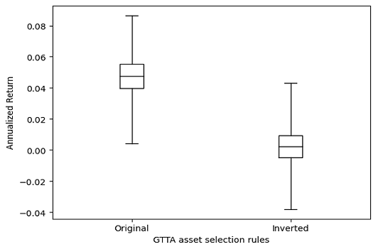
This kind of under-performance is exactly what is expected under the hypothesis that the GTTA strategy asset selection rules correspond to a true alpha signal.

Indeed, as Arnott et al.²⁶ puts it:

In inverting the strategies, we tacitly examine whether these strategies outperform because they are predicated on meaningful investment theses and deep insights on capital markets, or for reasons unrelated to the investment theses. If the investment beliefs are the source of outperformance, then contradicting those beliefs should lead to underperformance.

Trading strategy monitoring

Going beyond trading strategy evaluation, random portfolios can also be used to monitor how the performances of a trading strategy differ between in-sample and out-of-sample periods.

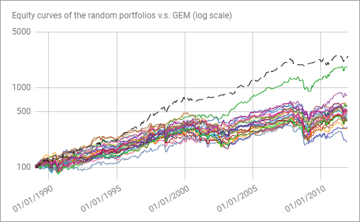
I propose to illustrate the associated process with another tactical asset allocation strategy, the Global Equities Momentum (GEM)⁴³ strategy of Gary Antonacci, which invests monthly - depending on the quantitative rules described in Antonacci⁴³ - in one asset among a three-asset universe made of:

• U.S. Equities, represented by the S&P 500 Index
• International Equities, represented by the MSCI ACWI ex-USA Index
• U.S. Bonds, represented by the Barclays Capital US Aggregate Bond Index

Because this strategy was published in 2013, let’s first check GEM performances during the in-sample period 1989-2012 (Google Sheet).

Figure 11 depicts the equity curves of a couple of random portfolios simulated⁴⁴ within Antonacci’s three-asset universe (in solid) v.s. the GEM equity curve (in dashed) over that period.

Figure 11. Global Equities Momentum (GEM) strategy v.s. random portfolios, in-sample period 1989-2012.

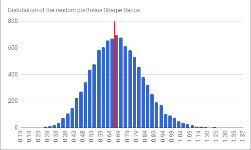
For the real thing, Figure 12 depicts the Sharpe Ratio distribution of 10000 random portfolios simulated⁴⁴ within Antonacci’s three-asset universe over that period, with the red line corresponding to the GEM Sharpe Ratio.

Figure 12. Global Equities Momentum (GEM) strategy v.s. random portfolios, distribution of Sharpe Ratios, in-sample period 1989-2012.

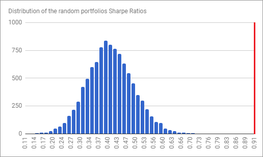
Pretty amazing, as the GEM Sharpe Ratio is among the best obtainable Sharpe Ratios over the in-sample period!

Let’s now check GEM performances during the out-of-sample period 2013-October 2020 (Google Sheet).

Figure 13 depicts the Sharpe Ratio distribution of 10000 random portfolios simulated⁴⁴ within Antonacci’s three-asset universe over that new period, with the red line again corresponding to the GEM Sharpe Ratio.

Figure 13. Global Equities Momentum (GEM) strategy v.s. random portfolios, distribution of Sharpe Ratios, out-of-sample period 2013-October 2020.

Pretty blah this time, with the GEM Sharpe Ratio roughly comparable to the median random portfolio Sharpe Ratio, which by definition exhibits no particular skill…

Such a difference in the GEM Sharpe Ratio relative to its simulated peer group¹ between the in-sample period and the out-of-sample period is puzzling, but analyzing a particular tactical asset allocation strategy is out of scope of this blog post, so that I need to leave the “why” question unanswered.

The same process can be applied to any trading strategy in order to detect a potential shift in that strategy’s performances, so, don’t hesitate to abuse the computing power available with today’s computers!

Conclusion

Dawson⁸ notes that [Monte Carlo analysis] is not a tool that has been readily applied to the investment process in the past, due to the perceived complexity of the problem⁸.

Through this blog post, I hope to have demonstrated that random portfolios are not necessarily complex to use, and come with many benefits for performance evaluation.

Feel free to randomly reach out on LinkedIn or on Twitter.

–

1. See Surz, Ronald, A Fresh Look at Investment Performance Evaluation: Unifying Best Practices to Improve Timeliness and Reliability, Journal of Portfolio Management, Vol. 32, No. 4, Summer 2006, pp 54-65. ↩ ↩² ↩³ ↩⁴ ↩⁵ ↩⁶ ↩⁷ ↩⁸ ↩⁹ ↩¹⁰ ↩¹¹ ↩¹² ↩¹³ ↩¹⁴

2. Or a trading strategy, or whatever. ↩

3. See Surz, R. J. 1994. Portfolio opportunity distributions: an innovation in performance evaluation. The Journal of Investing, 3(2): 36-41. ↩ ↩² ↩³ ↩⁴

4. See Surz, Ron. Accurate Benchmarking is Gone But Not Forgotten: The Imperative Need to Get Back to Basics, Journal of Performance Measurement, Vol. 11, No. 3, Spring, pp 34-43. ↩ ↩² ↩³

5. See Roberto Stein, Not fooled by randomness: Using random portfolios to analyse investment funds, Investment Analysts Journal, 43:79, 1-15. ↩ ↩² ↩³ ↩⁴ ↩⁵ ↩⁶ ↩⁷

6. By construction. ↩

7. These can be imposed by the firm that offers the funds, for example in terms of the prospectus and investment goals, or self-imposed trading behavior that the manager maintains over his career⁵; these can also be imposed by regulatory bodies or stock exchanges. ↩

8. See Dawson, R. and R. Young: 2003, Near-uniformly Distributed, Stochastically Generated Portfolios. In: S. Satchell and A. Scowcroft (eds.): Advances in Portfolio Construction and Implementation. Butterworth–Heinemann. ↩ ↩² ↩³ ↩⁴ ↩⁵ ↩⁶ ↩⁷ ↩⁸ ↩⁹

9. The $3$-dimensional geometrical object associated to the subset of $\mathbb{R}^3$ modeling long-only and full investment constraints is the standard 2-simplex in $\mathbb{R}^3$. ↩ ↩² ↩³

10. See Burns, P. (2007). Random Portfolios for Performance Measurement. In: Kontoghiorghes, E.J., Gatu, C. (eds) Optimisation, Econometric and Financial Analysis. Advances in Computational Management Science, vol 9. Springer, Berlin, Heidelberg. ↩ ↩² ↩³ ↩⁴ ↩⁵ ↩⁶

11. Such an object is also called a unit simplex or the probabilistic simplex. ↩

12. See Onn, S., Weissman, I. Generating uniform random vectors over a simplex with implications to the volume of a certain polytope and to multivariate extremes. Ann Oper Res 189, 331–342 (2011). ↩

13. See Kai-Tai Fang, Zhen-Hai Yang, On uniform design of experiments with restricted mixtures and generation of uniform distribution on some domains, Statistics & Probability Letters, Volume 46, Issue 2, 2000, Pages 113-120. ↩

14. See Paul A. Rubin (1984) Generating random points in a polytope, Communications in Statistics - Simulation and Computation, 13:3, 375-396. ↩

15. See Gert van Valkenhoef, Tommi Tervonen, Douwe Postmus, Notes on “Hit-And-Run enables efficient weight generation for simulation-based multiple criteria decision analysis”, European Journal of Operational Research, Volume 239, Issue 3, 2014, Pages 865-867. ↩

16. The rejection method is not a reasonable approach because the probability of a portfolio being accepted is generally extremely small when realistic constraints are in place¹⁰. ↩

17. Due to the nature of genetic algorithms. ↩

18. Within a given numerical tolerance. ↩

19. See Francesco Lisi (2011) Dicing with the market: randomized procedures for evaluation of mutual funds, Quantitative Finance, 11:2, 163-172. ↩ ↩² ↩³ ↩⁴ ↩⁵ ↩⁶ ↩⁷ ↩⁸

20. Some authors like Kritzman and Page³⁰ consider the usage of random portfolios to be a bootstrap simulation process, and not a Monte Carlo one. ↩

21. To be noted that the universe of assets, constraints and rules might perfectly be time-dependent; for example, at a given point in time, the universe of assets might be completely different from that at an earlier or later point in time. ↩

22. The frontier between the universe of assets and the rebalancing rules might not always be perfectly clear; at heart, the rebalancing rules must model the trading behaviour of the fund. ↩

23. See Kothari, S.P. and Warner, Jerold B., Evaluating Mutual Fund Performance (August 1997). ↩

24. See Ronald J. Surz, Testing the Hypothesis “Hedge Fund Performance Is Good”, The Journal of Wealth Management, Spring 2005, 7 (4) 78-83. ↩ ↩² ↩³ ↩⁴

25. See Burns, Patrick J., Performance Measurement Via Random Portfolios (December 2, 2004). ↩ ↩² ↩³

26. See Robert D. Arnott, Jason Hsu, Vitali Kalesnik, Phil Tindall, The Surprising Alpha From Malkiel’s Monkey and Upside-Down Strategies, The Journal of Portfolio Management, Summer 2013, 39 (4) 91-105. ↩ ↩² ↩³ ↩⁴

27. See N A Heard, P Rubin-Delanchy, Choosing between methods of combining p-values, Biometrika, Volume 105, Issue 1, March 2018, Pages 239–246. ↩

28. I have no affiliation. ↩ ↩²

29. See Molyboga, M., Ahelec, C. A simulation-based methodology for evaluating hedge fund investments. J Asset Manag 17, 434–452 (2016). ↩

30. See Kritzman, Mark and Sébastien Page (2003), The Hierarchy of Investment Choice, Journal of Portfolio Management 29, number 4, pages 11-23.. ↩ ↩² ↩³ ↩⁴ ↩⁵

31. See Staub, R. (2004). The Hierarchy of Investment Choice. The Journal of Portfolio Management, 31(1), 118–123. ↩

32. C.f. the MSCI World index factsheet. ↩

33. If future asset prices are available, for example thanks to a bootstrap simulation, nothing prevents a returns dispersion analysis to integrate them. ↩

34. In more details, the methodology is as follows: 1) Gross USD monthly price data for all the 23 countries represented in the MSCI World index has been collected from the MSCI website, 2) The MSCI World tracking portfolio - exhibiting a nearly null tracking error - has been computed over the period 31 December 2008 - 29 December 2023, which gives reference weights for the 23 countries represented in the MSCI World (e.g., United States ~50% and France ~5%), 3) Using Portfolio Optimizer, the evolution of 10000 random portfolios has been simulated over the period 31 December 2008 - 29 December 2023, these portfolios being a) constrained so that all country weights are positive, sum to one and all country weights except these for the United States and France are kept constant v.s. their reference weights and b) monthly rebalanced toward random portfolios in order to encompass any possible tilting, 4) The annualized return of each of these 10000 random portfolios has been computed. ↩

35. Which, in addition, is near the top of the achievable annualized returns! ↩

36. To be noted that in practice, this 95th quantile would probably need to be replaced by the 50th quantile because the benchmark return [should] always ranks median¹. ↩

37. (Adjusted) prices have have been retrieved using Tiingo. ↩

38. See Faber, Meb, A Quantitative Approach to Tactical Asset Allocation (February 1, 2013). The Journal of Wealth Management, Spring 2007. ↩ ↩² ↩³

39. In more details, using Portfolio Optimizer, the evolution of 25000 random portfolios has been simulated over the considered period, these portfolios being a) constrained so that all weights are positive and sum to a random exposure between 0% and 100% and b) monthly rebalanced toward random portfolios in order to encompass any possible tactical allocation. ↩

40. Which justifies a posteriori the use of the buy and hold portfolio as a benchmark. ↩

41. As a side note, Figure 9 highlights that an equal-weighted buy and hold portfolio is a tough benchmark to beat, c.f. DeMiguel et al.⁴⁵! ↩

42. Long-only and fully invested. ↩ ↩²

43. Gary Antonacci, Dual Momentum Investing: An Innovative Strategy for Higher Returns With Lower Risk ↩ ↩²

44. In more details, using Portfolio Optimizer, the evolution of 10000 random portfolios has been simulated over the considered period, these portfolios being a) constrained so that all weights are positive and sum to a 100% and b) monthly rebalanced toward random portfolios in order to encompass any possible tactical allocation. ↩ ↩² ↩³

45. See DeMiguel, Victor and Garlappi, Lorenzo and Uppal, Raman, Optimal Versus Naive Diversification: How Inefficient is the 1/N Portfolio Strategy? (May 2009). The Review of Financial Studies, Vol. 22, Issue 5, pp. 1915-1953, 2009. ↩