The Mathematics of Bonds: Simulating the Returns of Constant Maturity Government Bond ETFs
With more than $1.2 trillion under management in the U.S. as of mid-July 20221, investors are more and more using bond ETFs as building blocks in their asset allocation.
One issue with such instruments, though, is that their price history dates back to at best 20021, which is problematic in some applications like trading strategy backtesting or portfolio historical stress-testing.
In this post, which builds on the paper Treasury Bond Return Data Starting in 1962 from Laurens Swinkels2, I will show that the returns of specific bond ETFs - those seeking a constant maturity exposure to government-issued bonds - can be simulated using standard textbook formulas2 together with appropriate yields to maturity.
This allows in particular to extend the price history of these ETFs by several tens of years thanks to publicly available yield to maturity series published by governments, government-affiliated agencies, researchers…
Notes:
- A Google sheet corresponding to this post is available here
Mathematical preliminaries
Bond yield formula
In what comes next, I will make heavy use of the formula expressing the price of a bond as a function of its yield to maturity.
This formula can be found in the appendix A3.1 Yield to maturity for settlement dates other than coupon payment dates of Tuckman and Serrat3, and is reproduced below for convenience.
Le be a bond4 at a date $t$, with a remaining maturity equal to $T$, a yield to maturity equal to $y_t$ and a coupon rate equal to $c_t$.
Then, its price $P_t(c_t,y_t,T)$ per 100 face amount is equal to
\[\left( 1 + \frac{y_t}{2} \right)^{1 - \tau_{t}} \left[ \frac{100 c_{t}}{y_t} \left( 1 - \frac{1}{\left( 1 + \frac{y_t}{2} \right)^{2T}} \right) + \frac{100}{\left( 1 + \frac{y_t}{2} \right)^{2T}} \right] - 1\], where $\tau_{t}$ is the fraction of a semiannual period until the next coupon payment.
Par bond total return formula
Using the bond yield formula, it is possible to approximate the total return $TR$ of a par bond over a specific period using only its remaining maturity at the beginning of the period, its yield to maturity at the beginning of the period and its yield to maturity at the end of the period.
Par bond total return formula for a monthly period
In the case of a monthly period, let be a bond such that:
- Its remaining maturity at the end of the month $t-1$ is equal to $T$
- Its yield to maturity at the end of the month $t-1$, for a remaining maturity equal to $T$, is $y_{t-1}$
- Its yield to maturity at the end of the month $t$, for a remaining maturity equal to $T$, is $y_{t}$
Then, assuming that
- The bond trades at par at the end of the month $t-1$
- The bond yield curve at the end of the month $t$ is flat for remaining maturities between $T - \frac{1}{12}$ and $T$
, the total return $TR_t$ of this bond from the end of the month $t-1$ to the end of the month $t$ can be approximated by
\[\frac{y_{t-1}}{12} + \frac{y_{t-1}}{y_t} \left( 1 - \frac{1}{\left( 1 + \frac{y_t}{2} \right)^{2(T-\frac{1}{12})}} \right) + \frac{1}{\left( 1 + \frac{y_t}{2} \right)^{2(T-\frac{1}{12})}} - 1\]Demonstration of the par bond total return formula for a monthly period
A possible demonstration for the previous formula goes as follows.
At the end of the month $t-1$, the bond has the following characteristics:
- Its remaining maturity is equal to $T$
- Its coupon rate $c_{t-1}$ is equal to its yield to maturity $y_{t-1}$, because of the assumption that the bond trades at par at the end of the month $t-1$
Its price $P_{t-1}(c_{t-1},y_{t-1},T)$ is then equal, through the bond yield formula, to
\[100 \left( 1 + \frac{y_{t-1}}{2} \right)^{1 - \tau_{t-1}}\], with $\tau_{t-1}$ the fraction of a semiannual period until the next coupon payment at the end of month $t-1$.
At the end of the month $t$, the bond has the following characteristics:
- Its remaining maturity is equal to $T - \frac{1}{12}$, one month short of its initial remaining maturity $T$
- Its coupon rate $c_{t}$ is equal to $c_{t-1}$, that is, its initial yield to maturity $y_{t-1}$
- Its yield to maturity is equal to $y_{t}$, because of the assumption on the bond yield curve at the end of the month $t$
Its price $P_t(c_{t},y_{t},T - \frac{1}{12})$ is then equal, through the bond yield formula, to
\[\left( 1 + \frac{y_t}{2} \right)^{1 - \tau_{t}} \left[ \frac{100 y_{t-1}}{y_t} \left( 1 - \frac{1}{\left( 1 + \frac{y_t}{2} \right)^{2(T-\frac{1}{12})}} \right) + \frac{100}{\left( 1 + \frac{y_t}{2} \right)^{2(T-\frac{1}{12})}} \right]\], with $\tau_{t}$ the fraction of a semiannual period until the next coupon payment at the end of month $t$.
The total return $TR_t$ of this bond from the end of the month $t-1$ to the end of the month $t$ is then by definition equal to
\[\frac{P_t(c_{t},y_{t},T - \frac{1}{12})}{P_{t-1}(c_{t-1},y_{t-1},T)} - 1\], that is
\[\frac{\left( 1 + \frac{y_t}{2} \right)^{1 - \tau_{t}}}{\left( 1 + \frac{y_{t-1}}{2} \right)^{1 - \tau_{t-1}}} \left[ \frac{y_{t-1}}{y_t} \left( 1 - \frac{1}{\left( 1 + \frac{y_t}{2} \right)^{2(T-\frac{1}{12})}} \right) + \frac{1}{\left( 1 + \frac{y_t}{2} \right)^{2(T-\frac{1}{12})}} \right] - 1\]The first term of this expression corresponds to the re-investment of the accrued interest.
Under the practical assumptions that
- There is only a single rate for accrued interest, chosen equal to $y_{t-1}$5
- The accrued interest is not re-invested6
and noticing that $ \tau_{t} = \tau_{t-1} - \frac{1}{6}$7, this expression becomes
\[TR_t \approx \left[ \left( 1 + \frac{y_{t-1}}{2} \right)^{\frac{1}{6}} - 1 \right] + \left[ \frac{y_{t-1}}{y_t} \left( 1 - \frac{1}{\left( 1 + \frac{y_t}{2} \right)^{2(T-\frac{1}{12})}} \right) + \frac{1}{\left( 1 + \frac{y_t}{2} \right)^{2(T-\frac{1}{12})}} \right] - 1\]Finally, by linearizing the accrued interest through the first-order Taylor approximation $ \left( 1 + \frac{y_{t-1}}{2} \right)^{\frac{1}{6}} \approx \frac{y_{t-1}}{12} $, this expression becomes
\[TR_t \approx \frac{y_{t-1}}{12} + \left[ \frac{y_{t-1}}{y_t} \left( 1 - \frac{1}{\left( 1 + \frac{y_t}{2} \right)^{2(T-\frac{1}{12})}} \right) + \frac{1}{\left( 1 + \frac{y_t}{2} \right)^{2(T-\frac{1}{12})}} \right] - 1\]Remark:
Constructing return series for constant maturity government bonds
Methodology
Thanks to a variation9 of the par bond total return formula established in the previous section, Swinkels2 describes how to construct long (total) return series for government bonds using publicly available constant maturity government rates10.
These rates correspond to the yields to maturity of (fictitious) government bonds whose maturity is kept constant and are typically estimated by governments or government-affiliated agencies, which explains why they are publicly available. For example:
- In the U.S., they are called Constant Maturity Treasury Rates (CMTs), or Treasury Par Yield Curve Rates, and are published on:
- In France, they are called CNO-TEC and are published on the Banque de France website.
As a side note, long return series for government bonds are usually commercially licensed (Global Financial Data, Bloomberg…), so that the methodology of Swinkels2 participates to have a high-quality public alternative to commercially available data2 for research purposes.
Illustration
As an illustration of the methodology of Swinkels2, below are yields to maturity for 3 consecutive months taken from the FRED 10-Year Treasury Constant Maturity Rates series:
| Date | Yield to maturity |
|---|---|
| 31 Dec 2022 | 3.880% |
| 31 Jan 2023 | 3.520% |
| 28 Feb 2023 | 3.920% |
The total return series $ \left( TR_1, TR_2 \right) $ of the fictitious 10-year constant maturity government bond associated to these yields to maturity is then constructed by:
-
Computing the total return $TR_1$ from 31 Dec 2022 to 31 Jan 2023 thanks to the par bond total return formula, with $T = 10$, $y_{t-1} = 3.880\%$ and $y_t=3.520\%$.
This gives
\[TR_1 \approx \frac{0.0388}{12} + \frac{0.0388}{0.0352} \left( 1 - \frac{1}{\left( 1 + \frac{0.0352}{2} \right)^{2(10-\frac{1}{12})}} \right) + \frac{1}{\left( 1 + \frac{0.0352}{2} \right)^{2(10-\frac{1}{12})}} - 1\]That is
\[TR_1 \approx 3.31\%\] -
Computing the total return $TR_2$ from 31 Jan 2023 to 28 Feb 2023 thanks again to the par bond total return formula, but with this time $T = 10$11, $y_{t-1} = 3.520\%$ and $y_t=3.920\%$.
This gives
\[TR_2 \approx \frac{0.0352}{12} + \frac{0.0352}{0.0392} \left( 1 - \frac{1}{\left( 1 + \frac{0.0392}{2} \right)^{2(10-\frac{1}{12})}} \right) + \frac{1}{\left( 1 + \frac{0.0392}{2} \right)^{2(10-\frac{1}{12})}} - 1\]That is
\[TR_2 \approx -2.97\%\]
Implementation in Portfolio Optimizer
The Portfolio Optimizer endpoint /bonds/returns/par/constant-maturity implements the methodology of Swinkels2
using the par bond total return formula established in the previous section.
Simulating the returns of constant maturity government bond ETFs
Rationale
Many government bond ETFs target a specific maturity, a specific average maturity or a specific maturity range for their underlying portfolio of government bonds.
For example, the iShares 7-10 Year Treasury Bond ETF
seeks to track the investment results of an index composed of U.S. Treasury bonds with remaining maturities between seven and ten years12.
Intuitively, such ETFs should more or less behave like a constant maturity government bond, so that it should be possible to simulate their (total) returns using the methodology of Swinkels2 detailed in the previous section.
Nevertheless, and especially because these ETFs need to frequently rebalance their holdings13, such simulated returns might not be accurate enough to be of any practical use…
Let’s dig in.
Theory v.s. reality
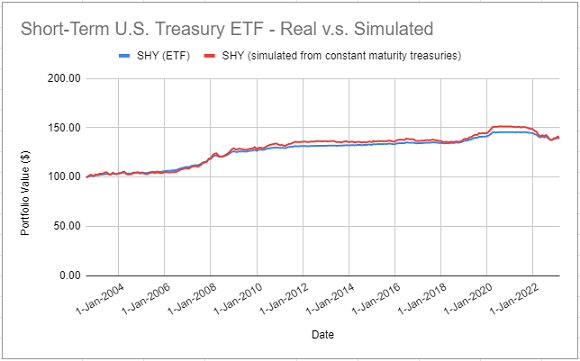
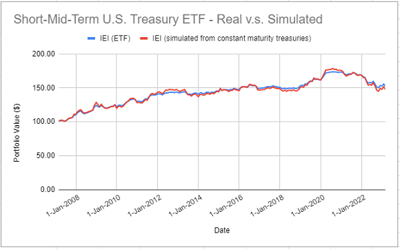
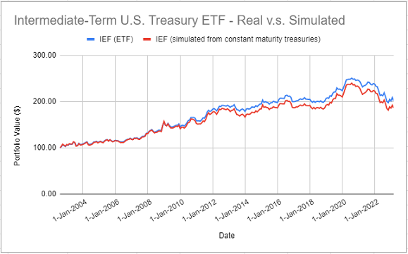
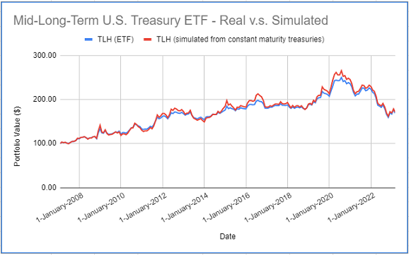
In order to illustrate the quality of the simulated returns discussed above, Figure 1 through Figure 5 compare the actual returns of the members of the iShares family of U.S. Treasury bond ETFs to the theoretical returns simulated using the methodology of Swinkels2.
- iShares 1-3 Year Treasury Bond ETF (SHY ETF)
The theoretical returns of this ETF are simulated with the FRED 3-Year Treasury Constant Maturity Rates.
- iShares 3-7 Year Treasury Bond ETF (IEI ETF)
The theoretical returns of this ETF are simulated with the FRED 7-Year Treasury Constant Maturity Rates.
- iShares 7-10 Year Treasury Bond ETF (IEF ETF)
The theoretical returns of this ETF are simulated with the FRED 10-Year Treasury Constant Maturity Rates.
- iShares 10-20 Year Treasury Bond ETF (TLH ETF)
The theoretical returns of this ETF are simulated with the FRED 20-Year Treasury Constant Maturity Rates.
- iShares 20+ Year Treasury Bond ETF (TLT ETF)
The theoretical returns of this ETF are simulated with the FRED 30-Year Treasury Constant Maturity Rates.
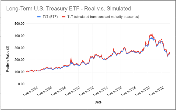
On all these figures, it is clear that simulated returns are closely matching actual returns.
The IEF ETF is an exception, though, because several simulated returns were significantly different from their actual counterparts over the period 2012 - 2014.
Nevertheless, for all the five ETFs, correlations between actual and simulated returns are greater than ~97%, which confirms that it is possible to accurately simulate the returns of constant maturity government bond ETFs14 using the methodology of Swinkels2.
Simulating the returns of non-constant maturity government bond ETFs
Each of the five ETFs analyzed in the previous section invests over a given segment of the U.S. Treasury yield curve (1-3 years, 3-7 years, 10-20 years…).
This segment is sometimes wide, like in case of the TLH ETF, but this characteristic allows these ETFs to be considered as constant maturity government bonds.
Now, what about non-constant maturity government bond ETFs?
To answer this question empirically, Figure 6 compares the actual returns of the iShares U.S. Treasury Bond ETF (GOVT ETF) to the
theoretical returns simulated using the methodology of Swinkels2 with a weighted average of 3-year, 7-year, 10-year, 20-year and 30-year Treasury constant maturity rates15.
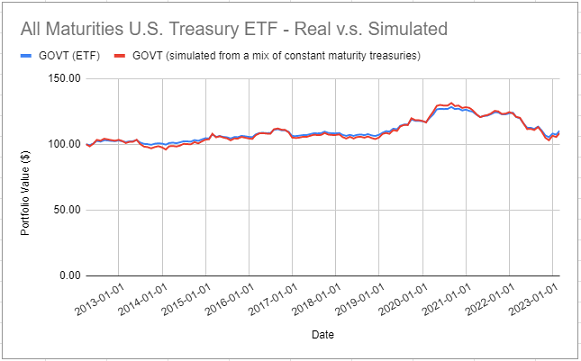
Once again, it appears that simulated returns are closely matching actual returns16.
This example shows that, at least in some cases, it should be possible to accurately simulate the (total) returns of non-constant maturity government bond ETFs using the methodology of Swinkels2, provided that these ETFs are considered as a weighted average of constant maturity government bonds instead of a single constant maturity government bond.
Extending the price history of constant maturity government bond ETFs
The previous sections demonstrated that it is possible to simulate quite accurately the returns of constant maturity government bond ETFs.
This opens the door to extending their price history.
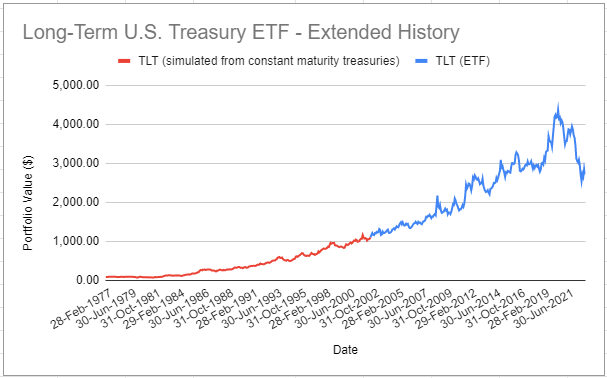
I will use the TLT ETF as an example.
Figure 5 showed that the actual returns of the TLT ETF are devilishly close to the theoretical returns simulated using the methodology of Swinkels2 with the FRED 30-Year Treasury Constant Maturity Rates series.
As a consequence, because the FRED provides the historical values of these rates back to February 1977, the price history of the TLT ETF can be extended by ~25 years.
This extended history is depicted in Figure 7.
Conclusion
This blog post described how to use the methodology of Swinkels2 to simulate present and past returns of constant maturity government bond ETFs.
One possible next step is to also use this methodology to simulate future returns of such ETFs, from views on future yields to maturity.
Maybe the subject of another post.
Meanwhile, feel free to connect with me on LinkedIn or follow me on Twitter to discuss about Portfolio Optimizer or about how to best approximate bond ETFs returns :-) !
–
-
See Swinkels, L., 2019, Treasury Bond Return Data Starting in 1962, Data 4(3), 91. ↩ ↩2 ↩3 ↩4 ↩5 ↩6 ↩7 ↩8 ↩9 ↩10 ↩11 ↩12 ↩13 ↩14 ↩15
-
See Tuckman, B., and Serrat A., 2022, Fixed Income Securities Tools for Today’s Markets, 4th edition, John Wiley And Sons Ltd. ↩
-
In this post, I use the same conventions as in Tuckman and Serrat3: bonds are assumed to be paying semiannual coupons, their coupon rate is assumed to be annual, their yield to maturity is assumed to be provided as semiannually compounded and their maturity is assumed to be expressed in years. ↩
-
Another sensible choice would be to use a rate equal to $\frac{y_{t-1} + y_{t}}{2}$. ↩
-
Since bonds with semi-annual coupons are paying coupons every six months, these coupons are anyway hardly collected and re-invested every month in practice, so that this is a sensible simplifying assumption. ↩
-
C.f. Tuckman and Serrat3 for explanations about the term $\frac{1}{6}$. ↩
-
See Swinkels, L., 2023, Historical Data: International monthly government bond returns, Erasmus University Rotterdam (EUR). ↩
-
C.f. the remark at the end of the previous section. ↩
-
Constant yield to maturity rates are frequently estimated from government bonds that trade close to par, even though interest rates have changed since their original issuance, which justifies the usage of this formula, c.f. Swinkels2. ↩
-
The maturity $T$ did not change because the bond is supposed to have a constant maturity. ↩
-
C.f. the iShares 7-10 Year Treasury Bond ETF website. ↩
-
For example, in order to target a specific maturity range, a government bond ETF must replace its holdings whose remaining maturity has become too short. As a side note, this behaviour explains the crazy annual portfolio turnover rate of these ETFs, with for example a turnover rate of 114% for the iShares 7-10 Year Treasury Bond ETF in 202217. ↩
-
Or at the very least, to accurately simulate the (total) returns of some constant maturity government bond ETFs. ↩
-
The weights correspond to the percentage breakdown of the GOVT ETF portfolio per maturity, retrieved from the iShares U.S. Treasury Bond ETF website on 19 March 2023. ↩
-
Numerically, correlation between actual and simulated returns is ~98%. ↩
-
C.f. the iShares 7-10 Year Treasury Bond ETF annual or semi-annual report. ↩