The Informativeness: Measuring the Homogeneity of a Universe of Assets
In this post, I will describe a measure of the homogeneity of a universe of assets, called the informativeness, introduced by Brockmeier et al.1 in their paper Quantifying the Informativeness of Similarity Measurements.
After quickly going through the associated mathematics, I will present two examples of usage of this measure - one as potential indicator of systemic risk and the other as as a means to choose between portfolio allocation methods.
Note: A Google sheet corresponding to this post is available here.
Mathematical preliminaries
Definition
Let be:
- $C \in \mathcal{M}(\mathbb{R}^{n \times n})$, $n \ge 2$, a correlation matrix
- $C_{\rho} \in \mathcal{M} \left( \mathbb{R}^{n \times n} \right)$, $\rho \in [-\frac{1}{n-1}, 1]$, an equicorrelation matrix2, with
Then, the raw3 informativeness of the correlation matrix $C$ is defined as its distance to the nearest equicorrelation matrix, that is
\[\textrm{informativeness}(\textup{C}) = \min_{\rho \in [-\frac{1}{n-1}, 1]} d(\textup{C},\textup{C}_\rho)\], where $d$ is any distance metric defined over the set of correlation matrices satisfying specific properties, like the Frobenius norm already used in the computation of the nearest correlation matrix.
More on the admissible distance metrics later.
Rationale
When all assets4 within a universe of assets have the same correlations, no pair of assets is more similar or dissimilar than any other pair5.
Running a hierarchical clustering algorithm in this universe will then not reveal any particular information about its structure, because no hierarchical grouping of the assets is appropriate.
Based on this observation, Brockmeier et al.1 define a non-informative correlation matrix to be an equicorrelation matrix, and define the informativeness of a correlation matrix to be the distance between that correlation matrix and the set of non-informative correlation matrices6.
With this definition of the informativeness:
- The lower the informativeness of a correlation matrix, the more homogeneous its correlations
- The higher the informativeness of a correlation matrix, the more heterogeneous its correlations, that is, the more nontrivial its correlation structure
Informativeness v.s. entropy
Information theory also provides a measure of the homogeneity (or of the lack of homogeneity) within an ensemble, known as entropy.
For example, the matrix effective rank is based on the Shannon’s entropy.
Brockmeier et al.1 emphasize that informativeness is different from entropy, and the differences between these two measures is best summarized by Figure 1, adapted from their paper.
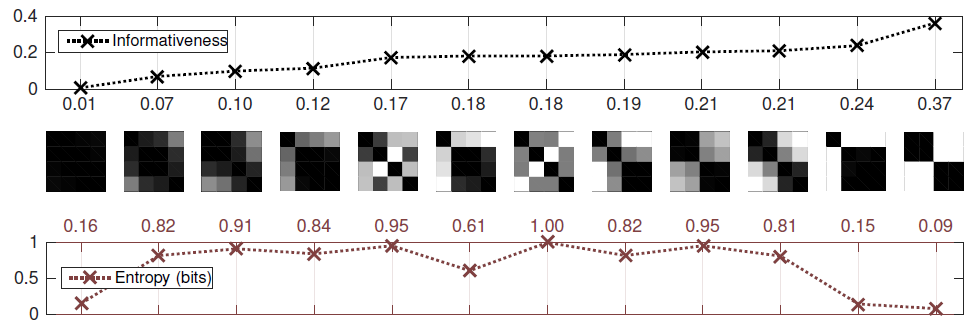
As noted by Brockmeier et al.1, Figure 1 shows that
informativeness is higher for nontrivial clusterings [of the objects], whereas entropy is maximized when [all objects are distinct]
Admissible distances
Not all distance metrics defined over the set of correlation matrices can be used to compute the informativeness.
An admissible distance metric $d$ must be:
- Invariant to symmetric permutations, that is,
, where $A$ and $B$ are correlation matrices and $\Pi$ is any permutation matrix, so that informativeness is invariant to the ordering of the assets4.
- Bounded, so that the raw informativeness can be normalized within the interval $[0,1]$
Brockmeier et al.1 compare the properties of several of such admissible distances, and conclude that they can be split in two groups exhibiting very different behaviour:
- Distances based on the Euclidean distance, like the Frobenius distance or the correlation matrix distance.
- Distances based on quantum information theory, like the Bures distance7
In particular, Brockmeier et al.1 establish empirically that
the three quantum-based distances (Chernoff bound, Quantum Hellinger and Bures) perform consistently well in identifying correlation matrices that are structured and more suitable for clustering
Implementation in Portfolio Optimizer
It is possible to compute the informativeness of a correlation matrix thanks to the Portfolio Optimizer API endpoint /assets/correlation/matrix/informativeness,
for which three different distance metrics are supported:
- The Frobenius distance $\mathcal{d}_F$ defined as
- The correlation matrix distance $\mathcal{d}_{corr}$ defined as
- The Bures distance $\mathcal{d}_{Bures}$ defined as
These distances have been selected based on the results of Brockmeier et al.1 mentioned in the previous section.
Examples of usage
Informativeness and stock market crashes
I will first illustrate the evolution of the informativeness of the U.S. stock market, thanks to the 49 industry portfolios of the Fama and French data library.
These 49 industries cover all stocks from the NYSE, the AMEX, and the NASDAQ, so that the associated informativeness should be representative of the U.S. stock market as a whole8.
I will use a rolling window approach, that is, at the end of each month I will:
- Compute the correlation matrix of the 49 industry portfolios over the last 12 months of monthly return data9
- Compute its informativeness10
Results for the period June 1970 - October 2022 are displayed in Figure 2, on which are also highlighted a handful of stock market crashes.
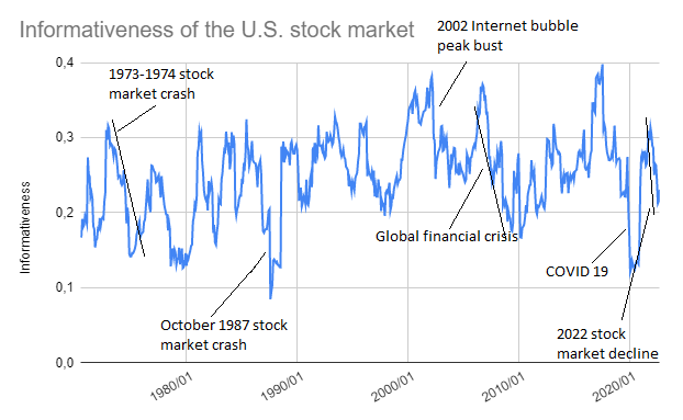
It appears that:
- The informativeness tends to drop during a stock market crash
Depending on the nature of the crash, the informativeness appears either to drop violently (e.g. October 1987 stock market crash, Internet bubble bust, Global Financial Crisis, COVID 19) or to drop over a time frame comparable with the stock market crash itself (e.g. 1973-1974 stock market crash, 2022 market decline).
- The informativeness tends to rebound strongly after a stock market crash, and this rebound usually coincides with the end of the crash
These observations suggest that the informativeness might be usable as an indicator of systemic risk11.
Informativeness as a means to choose between portfolio allocation methods
I will now study whether informativeness can help to predict the out-performance of the hierarchical risk parity portfolio (HRP) over a naive risk parity portfolio (NRP).
The motivation behind this study is the empirical link established by Brockmeier et al.1 between the informativeness and the performance of clustering algorithms.
For this, I propose to adapt the methodology used by Gautier Marti in his blog post Which portfolio allocation method to choose? Look at the correlation matrix! in order to evaluate how features extracted from a (in-sample) correlation matrix influence the (out-of-sample) volatility of portfolios constructed from this correlation matrix.
In details:
- I will use the Sector SPDR ETFs12 as the universe of assets
This universe of assets is again representative of the U.S. stock market as a whole, similar to the Fama-French 49 industry portfolios of the previous section, but the difference is that this time, this universe of assets is investable.
- I will use a rolling window approach over the ETF historical daily returns13.
At the end of each month, I will:
- In-sample, over the past 500 daily ETF returns
- Compute the ETF covariance matrix
- From it, compute both
- The NRP portfolio
- The HRP portfolio
- From it, extract the ETF correlation matrix and compute its informativeness14
- Out-of-sample, over the future 500 daily ETF returns
- Compute the realized annualized volatility of the NRP and HRP portfolios
The resulting relationship between the in-sample informativeness and the difference in the out-of-sample volatility of the NRP and HRP portfolios over the period December 2000 - December 2022 is represented in Figure 3.
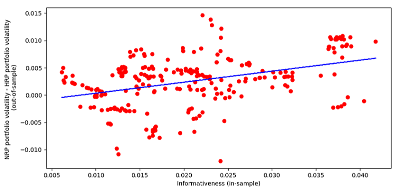
It seems that the higher the informativeness, the higher the volatility of the NRP portfolio in comparison with the HRP portfolio15.
Nevertheless, there are big flashing red lights:
- The values of the informativeness are very low, with a maximum of ~0.040 v.s. a theoretical maximum of 1
Such low values indicate that the universe of the Sector SPDR ETFs is actually too homogeneous to apply a hierarchical clustering algorithm on it.
So, whatever the relationship established, it is most probably spurious for this specific universe of assets.
The same study, using a more informative universe of assets, should allow to progress on this point.
- The differences in out-of-sample volatility between the two portfolios are very small
While it could be a consequence of the previous point, it could also mean that informativeness, as a stand alone correlation matrix feature, is not capable of predicting any economically significant out-performance16 of one portfolio allocation method v.s. the other.
But what if informativeness was used as an additional feature to the ones already discussed in Gautier Marti’s post above? Would it help?
Conclusion
Another possible usage of informativeness, similar in spirit to the unsupervised machine learning applications described in Brockmeier et al.1, would be to construct maximally informative universes of assets and study their properties.
For example, maybe these universes would be more stable, and so more predictable, than less informative universes?
Anyway, I hope that you enjoyed this last post of 2022 and that informativeness can find a place in your (quantitative) toolbox.
Happy end-of-year celebrations, and see you in 2023 for more research!
Meanwhile, you can connect with me on LinkedIn or follow me on Twitter to discuss about Portfolio Optimizer or quantitative finance in general.
–
-
See Austin J. Brockmeier and Tingting Mu and Sophia Ananiadou and John Y. Goulermas, Quantifying the Informativeness of Similarity Measurements, Journal of Machine Learning Research, 2017. ↩ ↩2 ↩3 ↩4 ↩5 ↩6 ↩7 ↩8 ↩9
-
For another example of usage of equicorrelation matrices, c.f. the post Correlation Matrix Stress Testing: Shrinkage Toward an Equicorrelation Matrix. ↩
-
Brockmeier et al.1 normalize the informativeness so that it belongs to the interval $[0,1]$. ↩
-
Although it might seem counterintuitive, even when all assets are totally uncorrelated there is no pair of assets that “stands out”, because in this case, all pairs of assets are similarly dissimilar. ↩
-
Another reasonable definition of the informativeness of a correlation matrix would be the distance between that correlation matrix and a particular equicorrelation matrix like an equicorrelation matrix made of 1s, but Brockmeier et al.1 explain why this definition would be wrong. ↩
-
Also known as the Bures–Wasserstein distance. ↩
-
To be noted, though, that working with industries v.s. with individual stocks imposes a structure on the U.S. stock market, which might artificially impact the value of the informativeness… ↩
-
The computed covariance matrix is thus not invertible, but this is not an issue for the computation of the informativeness. ↩
-
Using the Frobenius distance. ↩
-
My tests with other universes of assets representative of the U.S. stock market confirm that the evolution of the informativeness is a useful measure to monitor. What I couldn’t (yet) wrap my head around is whether the informativeness could be used as a stock market bottom indicator. I did not allocate as much time as I would have liked to this one and I am certainly lacking the proper mathematical tools, but I feel like it has potential… ↩
-
I will only use the 9 original sector ETFs, whose associated tickers are XLY, XLP, XLE, XLF, XLV, XLI, XLB, XLK and XLU. ↩
-
Adjusted for splits and dividends and retrieved thanks to Tiingo. ↩
-
Using the Bures distance, found in Brockmeier et al.1 to be able to identify correlation matrices suitable for clustering. Results using the two other distances implemented in Portfolio Optimizer are similar. ↩
-
And so, the higher the out-performance of the HRP portfolio, in terms of realized out-of-sample portfolio volatility. ↩
-
In terms of realized out-of-sample portfolio volatility. ↩