Trading Strategy Monitoring: Modeling the PnL as a Geometric Brownian Motion

Systematic trading strategies have the unfortunate habit of exhibiting worse performances in real-life than in backtests, partially due to backtest overfitting¹.

Monitoring their behavior once they are deployed in production is then very important to be able to detect as early as possible any inconsistency between their live returns and their expected returns.

For this, I will describe in this blog post the methodology proposed by Rej et al.² in their paper You are in a drawdown. When should you start worrying?, which consists in comparing the current drawdown of a trading strategy with the theoretical drawdown that would be expected under the assumption that the profit and loss (PnL) of the strategy is modeled as a geometric Brownian motion.

Using this methodology, I will analyze the drawdowns of the U.S. stock market over the past ~150 years and I will show how the geometric Brownian motion model could be used in a risk management strategy to scale the market exposure of a portfolio of U.S. equities.

Mathematical preliminaries

The joint probability density of the length and of the depth of the current drawdown of a trading strategy

Let be:

• $[0, T]$ a finite time interval, measured in years
• $\mathrm{PnL}(t), 0 \leq t \leq T$, the PnL of the trading strategy over the interval $[0, T]$
• $\mathrm{SR}$, the annualized Sharpe ratio of the trading strategy

Then, assuming that:

• $\mathrm{PnL}$ is appropriately modeled by a geometric Brownian motion over the interval $[0, T]$, with annualized drift $\mu$ and annualized volatility $\sigma$
• $\sigma$ is normalized to $\sigma = 1$

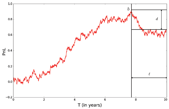
Rej et al.² build on the results from Shepp³ to establish that the joint probability density for the PnL of the trading strategy to reach a maximum $b$ at time $T - l$ and subsequently suffers a drawdown of depth $d$ is given by

\[\tilde{F}(d,b,l) = \frac{bd}{\pi \left( (T-l) l \right )^{\frac{3}{2}}} e^{ \left ( \mathrm{SR} (b-d) - \mathrm{SR}^2 \frac{T}{2} - \frac{d^2}{2l} - \frac{b^2}{2(T-l)} \right ) }\]

where $d$ is defined by

\[d = \ln \left( \max_{0 \leq t \leq T} \mathrm{PnL(t)} \right) - \ln \left( \mathrm{PnL}(T) \right)\]

The quantities $b$, $l$, and $d$ are illustrated in Figure 1, adapted from Rej et al.²

Figure 1. Illustration of the quantities appearing in the formula for $\tilde{F}$. Source: Rej et al.

The formula for $\tilde{F}$ is consistent with the empirical findings of Van Hemert et al.⁴ in a more realistic setting, who remark that:

Key drivers of the maximum drawdown […] are the evaluation horizon (time to dig a hole), Sharpe ratio (ability to climb out of a hole), and persistence in risk (chance of having a losing streak).

It follows from this formula that the joint probability density of the length $l$ and of the depth $d$ of the current drawdown of the trading strategy is given by

\[G(l, d) = \int_{0}^{+\infty} \tilde{F}(d,b,l) \mathrm{d}b\]

To be noted that in case $\sigma$ is not normalized to $\sigma = 1$⁵:

• Either the formula for $\tilde{F}$ needs to be corrected using the results from Shepp³
• Or the formula for $d$ needs to be normalized, with $d$ becoming the dollar amount of drawdown divided by the annualized dollar volatility² defined by

\[d = \frac{\ln \left( \max_{0 \leq t \leq T} \mathrm{PnL(t)} \right) - \ln \left( \mathrm{PnL}(T) \right)}{\sigma}\]

Derived probability densities

Using the formula for $G$, Rej et al.² explicitly derive:

• The probability density of the length of the current drawdown, defined as

\[\rho(l) = \int_{0}^{+\infty} G(u,l) \mathrm{d}u\]

• The probability density of the depth of the current drawdown, defined as

\[\psi(d) = \int_{0}^{T} G(d,l) \mathrm{d}l\]

In addition, it is also possible to derive the conditional density of:

• The length of the current drawdown having observed its depth $d^*$

\[\eta(l|\mathrm{d^*}) = \frac{G(\mathrm{d^*},l)}{\psi(\mathrm{d^*})}\]

• The depth of the current drawdown having observed its length $l^*$

\[\gamma(d|\mathrm{l^*}) = \frac{G(d,\mathrm{l^*})}{\rho(\mathrm{l^*})}\]

These probability densities allow to answer questions like:

• (Strategy monitoring) With 95% confidence, is the length or depth of the current drawdown of a trading strategy compatible with the assumption that its Sharpe ratio is $\mathrm{SR_{ref}}$?
• (Risk management) What is the probability that the current drawdown of a trading strategy of Sharpe ratio $\mathrm{SR_{ref}}$ lasts more than $\mathrm{t_{ref}}$ years, knowing that its current depth is $d^*$?

Remarks on the Brownian motion assumption

The assumption made in Rej et al.² that the PnL of the trading strategy follows a geometric Brownian motion might appear unrealistic in practice since financial returns are far from being Gaussian⁶.

Nevertheless, two remarks about this model:

• Aggregational Gaussianity⁷ is as much a stylized fact of financial returns than non-Gaussianity⁶.

  So, depending on the observation frequency of the trading strategy (monthly, quarterly, yearly…), a geometric Brownian motion model could be good enough for coarse monitoring purposes.

• Non-normality, heteroskedasticity, etc. of financial returns all increase the severity of the drawdowns of a trading strategy²⁴.

  From this perspective, a geometric Brownian motion model represents an over-optimistic reference model, which can be used to set minimal (or maximal) expectations.

As Rej et al.² put it:

we argue that from a practitioner’s point of view, it is always better to err on the side of caution, so that the Brownian model sets a very useful benchmark.

Implementation in Portfolio Optimizer

Portfolio Optimizer does not provide any API endpoint to compute the probability distributions mentioned in the previous section, but provides access - through the endpoint /markets/indicators/pcdenw/us - to the Probability of Current Drawdown Ending Next Week indicator detailed in the next section for the U.S. stock market.

Examples of application

I will present two examples of application of the methodology of Rej et al.², slightly out of the context of trading strategy monitoring.

Analysis of the U.S. stock market historical drawdowns

In this first example of application, I will analyze the drawdowns of the U.S. stock market over the past ~150 years and determine which insights (if any) can be gained from the geometric Brownian motion model.

Data

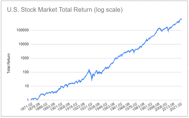
I will use the U.S. stock market monthly returns⁸ over the period January 1871 - September 2022 available on Robert J. Shiller’s website, whose PnL is depicted in Figure 2.

Figure 2. U.S. stock market total return, January 1871 - September 2022.

Sharpe ratio

Over the whole period January 1871 - September 2022, the annualized Sharpe ratio of the U.S. stock market is ~0.65-0.69, depending on the type of monthly returns used (simple v.s. log).

To be conservative, I will select $\mathrm{SR_{US}} = 0.65$.

Length and normalized depth of historical drawdowns

Computing the length of historical drawdowns is straightforward.

On the other hand, computing the normalized depth of historical drawdowns requires an estimate of the volatility $\sigma_{US}$ of the geometric Brownian motion.

I will simply take $\sigma_{US} = 14$%, which corresponds to the annualized volatility of the U.S. stock market over the whole period January 1871 - September 2022 that I already used in the estimation of the Sharpe ratio $\mathrm{SR_{US}}$.

Probability distributions of the length and of the depth of the current drawdown

The probability densities $\rho$ and $\psi$ allow to compute the probability distribution functions of the length and of the normalized depth of the current drawdown for the U.S. stock market, with $T = \frac{1821}{12} \approx 152$ years.

They are displayed in Figure 3 and 4.

Figure 3. Probability distribution of the length of the current drawdown for the U.S. stock market.

Figure 4. Probability distribution of the normalized depth of the current drawdown for the U.S. stock market.

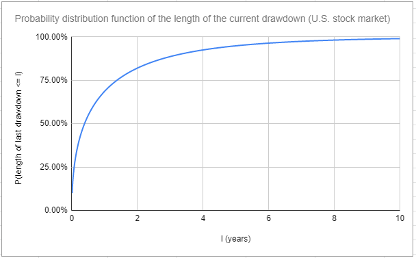
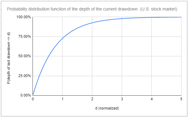
It follows that when the U.S. stock market is in a drawdown, then, with a confidence of ~95%:

• This drawdown will last less than ~5 years
• The normalized depth of this drawdown will be lower than ~2.25, which corresponds to a drawdown percentage of ~27%

I will rephrase this.

Under an over-optimistic model, a current drawdown of up to ~27% or lasting up to ~5 years needs to be considered business as usual⁹ for the U.S. stock market.

I was honestly surprised by this result, which matches with the comment from Rej et al.²:

[…] investors tend to underestimate the length and depth of perfectly acceptable, “normal” drawdowns.

By the way, it is possible to confirm that the geometric Brownian motion model is indeed over-optimistic, because it underestimates the characteristics of the major historical drawdowns.

Two examples:

• (Dot-Com Bubble) The length of the drawdown from May 2000 to September 2006 had an a ~0.035% probability of occurring
• (Global Financial Crisis) The normalized depth of the drawdown from November 2007 to July 2012 had a ~0.002% probability of occurring

Confidence interval for the conditional length of the current drawdown

Borrowing the idea of Rej et al.², the conditional probability density $\eta$ allows to compute a confidence interval $[l^-, l^+]$ for the length $l$ of the current drawdown conditional on its normalized depth $\mathrm{d^*}$, such that

\[\mathbb{P} \left( l^- \leq l \leq l^+ | \mathrm{d^*} \right) = 1 - \alpha\]

with $1 - \alpha \in [0,1] $ a given confidence level (90%, 95%…).

Such a conditional confidence interval for the U.S. stock market, at the 95% level, is displayed in Figure 5.

Figure 5. 95% confidence interval for the length of the current drawdown for the U.S. stock market having observed its normalized depth.

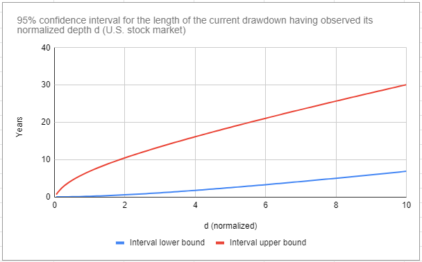
Now, if we compare the length of historical drawdowns to the conditional confidence interval of Figure 5, it appears that these lengths are usually much closer from the lower boundary of the conditional confidence interval than from its upper boundary.

Two examples again:

• (Dot-Com Bubble) This drawdown of normalized depth ~3.84 lasted 6.08 years, while its 95% conditional confidence interval is $[1.64, 15.71]$ years
• (COVID-19) This drawdown of normalized depth ~1.50 lasted 0.42 years, while its 95% conditional confidence interval is $[0.34, 8.78]$ years

This over-pessimistic conditional confidence interval is in stark contrast to the over-optimistic probabilities of the previous section.

Thus, there is something really interesting happening here, which might have practical implications for investors.

For example, using history as a guide, an investor could think that because the length of the most severe drawdown for the U.S. stock market has been ~15 years¹⁰, she needs to prepare, worst case, for a future drawdown of about ~15 years.

Problem is, the 95% conditional confidence interval for the length of a drawdown as severe as the said drawdown¹¹ is $[9.00, 34.67]$ years, implying that this investor actually needs to prepare for a future drawdown of up to ~35 years¹²!

Managing the exposure of a portfolio of U.S. equities

In this second example of application, I will investigate how to use the geometric Brownian motion model to scale the market exposure of a portfolio of U.S. equities in case the U.S. stock market is in a drawdown.

Specifically, I propose to analyze the following risk management strategy.

At the end of each week:

• If the U.S. stock market is in a drawdown of sufficient normalized depth¹³
  • Compute the conditional probability that this drawdown ends by the next week, which results in a probability $p$ from 0% to 100%
  • Allocate $p$% of the portfolio to U.S. equities and $1-p$% to cash
• Otherwise, allocate 100% of the portfolio to U.S. equities

Figure 6 illustrates this strategy with the SPY ETF (U.S. equities) and the SHY ETF (cash) over the period January 1993 - November 2022¹⁴, and compare it to a buy and hold strategy over the same period.

Figure 6. Buy and hold v.s. drawdown probability-adjusted SPY.

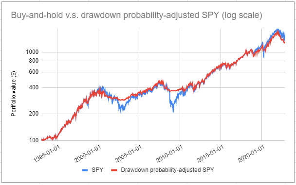
A quick visual inspection of Figure 6 shows that this strategy seems to be able to limit the severity of drawdowns while matching the raw performances of the U.S. stock market.

Some statistics:

Portfolio Management Strategy	Average Exposure	Annualized Sharpe Ratio	Maximum (Weekly) Drawdown
Buy and hold	100%	~0.61	~55%
Drawdown probability-adjusted	~83%	~0.75	~25%

What I find interesting with this strategy is that it is a kind of momentum strategy, but not based on the usual momentum indicators (moving averages, rate of change…).

So, it might be a useful addition to one’s arsenal.

Geek notes:

• I made $T$ dynamic in order to mimic a real-time execution of this strategy; the initial value of $T$ is ~122 years, and with each passing week its value is incremented by $\frac{1}{52}$
• I re-used the Sharpe ratio $SR_{US}$ of 0.65 and the volatility $\sigma_{US}$ of 14%; this does not introduce any lookahead bias because these values computed over the whole period January 1871 - September 2022 are nearly identical to their counterparts computed over the period January 1871 - December 1992
• If the Sharpe ratio and/or the volatility are made dynamic, for example estimated from a rolling window of past returns, much better performances could be obtained; this goes a little beyond the static model of Rej et al.² though

Conclusion

There are of course many other possibilities to use the methodology of Rej et al.².

One such possibility, again in risk management, could be for example to compute the probability that the depth of the current drawdown worsens having observed its current length, and de-risk a portfolio accordingly.

That’s all for now!

As usual, you can connect with me on LinkedIn or follow me on Twitter to discuss about Portfolio Optimizer or quantitative finance in general.

–

1. See David H. Bailey, Jonathan M. Borwein, Marcos Lopez de Prado and Qiji Jim Zhu, The probability of backtest overfitting, Journal of Computational Finance, VOLUME 20, NUMBER 4 (APRIL 2017) PAGES: 39-69 or the SSRN version. ↩

2. See A. Rej, P. Seager and J.-P. Bouchaud, You are in a drawdown. When should you start worrying?, Wilmott, Volume 2018, Issue 93, January 2018, Pages 56-59 or the arXiv version. ↩ ↩² ↩³ ↩⁴ ↩⁵ ↩⁶ ↩⁷ ↩⁸ ↩⁹ ↩¹⁰ ↩¹¹ ↩¹² ↩¹³

3. See Shepp, L. 1979. The joint density of the maximum and its location for a Wiener process with drift. Journal of Applied Probability 16(2), 423–427. ↩ ↩²

4. See Drawdowns, Otto Van Hemert, Mark Ganz, Campbell R. Harvey, Sandy Rattray, Eva Sanchez Martin and Darrel Yawitch, The Journal of Portfolio Management September 2020. ↩ ↩²

5. Which is probably the most usual situation in practice… ↩

6. See R. Cont (2001) Empirical properties of asset returns: stylized facts and statistical issues, Quantitative Finance, 1:2, 223-236. ↩ ↩²

7. Aggregational Gaussianity refers to the tendency of asset returns to follow a distribution closer and closer to a Gaussian distribution the more the time period over which they are computed increases. ↩

8. The monthly returns are total nominal returns (i.e., the consumer price index was forced to 1 in Shiller’s Excel sheet to explicitly discard inflation). ↩

9. In particular, such a drawdown does not require any exogenous explanation (pandemic, recession, war…). ↩

10. January 1929 - December 1944. ↩

11. Whose normalized depth is 12.15407251. ↩

12. In this context, markets can remain irrational longer than you can remain solvent is a perfectly appropriate quote. ↩

13. As a definition of sufficient, I choose a drawdown whose normalized depth is such that its probability of occurrence under the geometric Brownian motion model is greater than or equal to 66% (i.e., the two third quantile of the probability distribution of the normalized depth of the current drawdown). ↩

14. SPY and SHY adjusted close prices were retrieved from Tiingo, and SHY history wasz extended with index data. ↩