The Diversification Ratio: Measuring Portfolio Diversification
Continuing the series of blog posts on diversification indicators, I describe in this post a correlation-based measure of portfolio diversification called the diversification ratio, initially introduced by Yves Choueffaty and Yves Coignard in their paper Toward maximum diversification1 and later extensively studied in other papers from people at Think Out of the Box Asset Management (TOBAM)23.
I first detail the mathematics associated to the diversification ratio and I then present a few of its possible uses in both portfolio analysis and portfolio optimization.
Notes:
- A Google sheet corresponding to this post is available here
Mathematical preliminaries
Let be:
- $n$, the number of assets in a universe of assets
- $w = (w_1,…,w_n) \in {\mathbb{R}^*}^{n}$, the asset weights of a portfolio invested in the considered universe of assets
- $\Sigma \in \mathcal{M}(\mathbb{R}^{n \times n})$, the asset covariance matrix
- $\sigma = (\sigma_1,…,\sigma_n) \in {\mathbb{R}^+}^{n}$, the asset volatilities
Diversification ratio
Definition
The diversification ratio $DR(w)$ of a portfolio with asset weights $w$ is the ratio of the weighted average of the asset volatilities to the portfolio volatility1, that is
\[DR(w) = \frac{ \sigma{}^t w}{\sqrt{ w {}^t \Sigma w }}\]Interpretation
Choueifaty et al.2 show that the diversification ratio can be decomposed into an asset correlation component and an asset weight component, and that the diversification ratio increases (resp. decreases) when:
- The concentration in asset weights decreases (resp. increases)
- The average correlation between assets decreases (resp. increases)
From this perspective, the diversification ratio can be interpreted as a correlation-based measure of portfolio diversification consistent with the intuition that portfolios with concentrated weights and/or highly correlated holdings would be poorly diversified2, whatever the exact measure of diversification used4.
Most diversified portfolio
Definition
- The (long-only) most diversified portfolio (MDP) is the long-only and fully invested portfolio which maximizes the diversification ratio1, that is, the portfolio whose asset weights $w_{MDP}$ satisfy
- The long-short most diversified portfolio (LSMDP) is the long-short and fully invested portfolio which maximizes the diversification ratio13, that is, the portfolio whose asset weights $w_{LSMDP}$ satisfy
-
The constrained most diversified portfolio is the portfolio whose asset weights $w_{CMDP}$ satisfy
\[w_{CMDP} = \operatorname{argmax} \frac{w {}^t \sigma }{\sqrt{ w {}^t \Sigma w}} \textrm{s.t. } w \in S\], where $S$ is a subset of $\mathbb{R}^n$ representing asset weight constraints like full-investment constraint, long-only constraint, maximum and minimum weight constraints, etc.
Choueifaty et al.12 demonstrate that the most diversified portfolio and the long-short most diversified portfolio always exist and are both unique if the covariance matrix $\Sigma$ is invertible5.
Similarly, under reasonable assumptions6, it can be demonstrated that the constrained most diversified portfolio always exists and is unique if the covariance matrix $\Sigma$ is invertible.
Rationale
Risk-based portfolio construction methods7, to which the most diversified portfolio belongs, grew in popularity after the Global Financial Crisis of 2007-2008, during which many portfolios allocation strategies that were supposed to be well-diversified4 failed to deliver the promised diversification benefits.
The most diversified portfolio aims to deliver investors the full benefit of the equity premium2 by avoiding in particular the concentration risk associated with market capitalization-weighted portfolios.
The name of this portfolio might be misleading, though, because it is by definition the portfolio which maximizes the diversification ratio, but nothing can be said in general about its maximization properties related to other measures of diversification.
As Lee8 puts it:
In other words, it cannot be ruled out that the MDP that maximizes […] the diversification ratio can itself be a relatively concentrated portfolio that is not as diversified when judged by other definitions of diversification.
Properties
Choueifaty et al.12 establish the following core properties9:
Property 1: The long-short most diversified portfolio has the same (strictly) positive correlation $\frac{1}{DR \left( w_{LSMDP} \right) }$ with all the assets.
Property 2: The most diversified portfolio has the same (strictly) positive correlation $\frac{1}{DR \left( w_{MDP} \right) }$ with all the assets that have a non-null weight in that portfolio. Additionally, any null-weighted asset is more correlated to the most diversified portfolio than any non null-weighted asset.
Froidure et al.3 establish several other properties, among which:
Property 3: The most diversified portfolio is the portfolio, among all long-short portfolios, that maximizes its minimal correlation with all the assets, with all the long-only portfolios and with all the long-only factors10.
Property 4: The most diversified portfolio is the portfolio, among all long-only portfolios, that is the most correlated with the long-short most diversified portfolio.
Property 5: The most diversified portfolio is stable11, in that a small12 perturbation in the asset covariance matrix results in a small perturbation in the most diversified portfolio asset weights.
And other authors have also contributed to the analysis of the most diversified portfolio:
- Clarke et al.13, who find an analytic solution for the asset weights of the most diversified portfolio under a single-factor model and use it to explain why only a small proportion of assets within a universe of assets has non-null weights in the most diversified portfolio14
- Carmichael et al.15, who show that the most diversified portfolio minimizes portfolio variance subject to a diversification constraint, where diversification is measured by Rao’s quadratic entropy16, which addresses initial concerns about the lack of clarity of the investment problem that the most diversified portfolio is supposed to solve817.
- …
Correlation spectrum
Definition
The correlation spectrum of a portfolio is the $n$-dimensional vector made of the correlation of that portfolio with all the $n$ assets3.
More formally, the correlation spectrum of a portfolio with asset weights $w$ is the vector $\rho(w) \in [-1,1]^n$ satisfying
\[\rho(w)_i = \frac{ e_i {}^t \Sigma w }{\sqrt{ w {}^t \Sigma w } \sqrt{ e_i {}^t \Sigma e_i }} , i=1..n\], where $e_i \in \mathbb{R}^n$ is the i-th vector of the canonical basis of $\mathbb{R}^n$, representing the single-asset portfolio fully invested in the asset i.
Rationale
Froidure et al.3 note that the weight of an asset in a portfolio does not in general reflect to which extent the portfolio is exposed to that particular asset.
As an example, Figure 1 compares the evolution of two portfolios invested in the universe of the 11 S&P Sectors represented by the 11 Sector SPDR ETFs, over the year 2022:
- A portfolio $P_{SPDRs}$, with non-null asset weights on the Consumer Discretionary, Health Care, Materials, Technology and Utilities sectors and null asset weights on all the other sectors
- A portfolio $P_{XLRE}$, with a 100% asset weight on the Real Estate sector
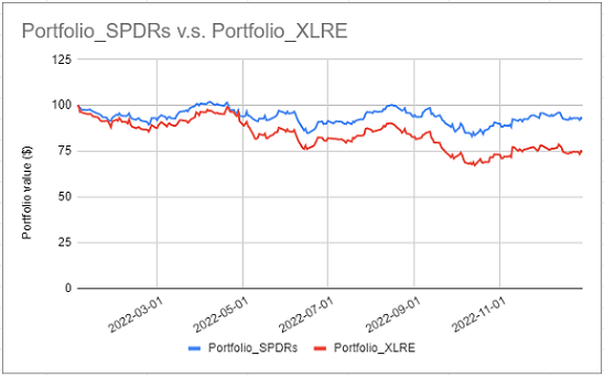
From this figure, as well as from the correlation of these two portfolios18, the exposure of the portfolio $P_{SPDRs}$ to the Real Estate sector is actually far from null despite not being invested at all in this sector!
The correlation spectrum aims to solve this shortcoming of asset weights and to unveil the effective exposure of a portfolio, in terms of correlations, to all the assets in a universe of assets.
Properties
The main property of the correlation spectrum is3:
Property 6: The correlation spectrum is a correlation-based representation of a long-short portfolio that is fully equivalent, up to leverage, to the representation of a portfolio in terms of asset weights.
This property allows to work interchangeably with the representation of a portfolio in terms of asset correlations or in terms of asset weights, depending on whatever representation is better suited to a given context.
Rho-representativity
Definition
A portfolio with asset weights $w$ is said3 to be rho-representative19 if its correlation spectrum $\rho(w)$ is such that $\rho(w)_i > 0$, $i=1..n$.
In other words, a rho-representative portfolio is (strictly) positively exposed, in terms of correlations, to all the assets in a universe of assets.
Properties
While investigating misc. properties related to rho-representativity, Froidure et al.3 derive the following major relationship between any long-only portfolio and the diversification ratio of the most diversified portfolio:
Property 7: A long-only portfolio is (strictly) positively correlated to at least one asset, a lower bound for this correlation being $\frac{1}{DR \left( w_{MDP} \right)^2}$.
They also examine the rho-representativity of several well known portfolios, and conclude that:
- The most diversified portfolio is rho-representative
- The long-only equal risk contributions portfolio (ERC) is rho-representative
- The long-only minimum-variance portfolio (MV) is rho-representative
- The equal-weighted portfolio (EW) and the market capitalization-weighted portfolio (MKT) are not necessarily rho-representative
Implementation in Portfolio Optimizer
Portfolio Optimizer implements several endpoints related to the diversification ratio:
- Computation of the diversification ratio of a portfolio, both from its definition in the previous section and from time series20, through the endpoint
/portfolios/analysis/diversification-ratio - Computation of the correlation spectrum of a portfolio, both from its definition in the previous section and from time series, through the endpoint
/portfolios/analysis/correlation-spectrum - Computation of the (linearly constrained) most diversified portfolio, through the endpoint
/portfolios/optimization/most-diversified
Examples of usage of the diversification ratio in portfolio analysis
Measuring portfolio diversification
The most natural way to use the diversification ratio is to assess the level of diversification of a specific portfolio.
For instance, re-using the universe of the 11 S&P Sectors introduced in the previous section:
- Figure 2 displays the asset weights of the minimum variance portfolio
- Figure 3 displays the asset weights of a diversified near-minimum variance portfolio
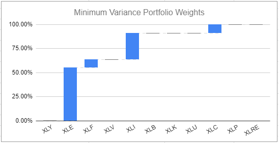
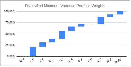
The diversified near-minimum variance portfolio is visibly less concentrated in terms of asset weights than the minimum variance portfolio and should intuitively be more diversified.
Computing the diversification ratio confirms this intuition21:
| Portfolio | Diversification ratio |
|---|---|
| Minimum variance | ~1.18 |
| Diversified near-minimum variance | ~1.24 |
Determining the number of independent risk factors represented in a portfolio
Choueifaty et al.2 observe that:
- The diversification ratio of a long-only portfolio is equal to 1 when the portfolio is a single-asset portfolio
- The diversification ratio of a long-only portfolio is equal to $\sqrt n$ when the portfolio is an equal-weighted portfolio of $n$ uncorrelated assets with identical volatility
Based on these observations, they propose to interpret the squared diversification ratio of a portfolio $DR(w)^2$ as the effective number of independent risk factors, or degrees of freedom, represented in the portfolio2, which makes it very similar to another measure of portfolio diversification called the effective number of bets and introduced by Meucci22.
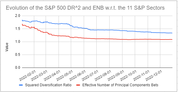
In order to empirically validate this interpretation, I propose to estimate the number of independent risk factors represented in the S&P 500 using both:
- The daily one year23 rolling squared diversification ratio
- The daily one year rolling effective number of principal components bets24
of the portfolio $P_{SPY}$ reproducing the S&P 500 within the universe of the 11 S&P Sectors25.
Results are displayed in Figure 4, in which it indeed appears that the general behavior of these two measures is comparable, with a severe decrease over the whole year 2022.
However, one issue with the interpretation of $DR(w)^2$ as the number of independent risk factors represented in a portfolio is that $DR(w)^2$ is unbounded26 due to the diversification ratio itself being unbounded.
This is easily established in the case of two assets, where the diversification ratio of an equal-weighted portfolio of two assets with a pairwise correlation $\rho$ and with an identical volatility equals $\sqrt { \frac{2}{1 + \rho} }$, which goes to infinity as $\rho$ goes to -1.
More on this a little bit later.
Analyzing the amount of available diversification not utilized in a portfolio
A consequence of the previous paragraph is that comparing the squared diversification ratio of a portfolio $DR(w)^2$ to the squared diversification ratio of the most diversified portfolio $DR(w_{MDP})^2$ enables to analyze the amount of untapped diversification27 of that portfolio in terms of exposures to independent risk factors within a universe of assets.
This kind of analysis is used in practice by people at TOBAM28.
When applied to the universe of the 11 S&P Sectors, it gives:
| Portfolio | Portfolio squared diversification ratio | MDP squared diversification ratio | Available diversification used by the portfolio | Available diversification not used by the portfolio |
|---|---|---|---|---|
| $P_{SPY}$ | ~1.33 | ~1.81 | ~74% | ~26% |
Quantifying how diversified is a universe of assets
From Property 7, the minimal correlation between a long-only portfolio invested in a universe of assets and at least one asset in that universe is equal to the inverse of the squared diversification ratio of the most diversified portfolio, $\frac{1}{DR \left( w_{MDP} \right)^2}$.
This property allows to interpret $\frac{1}{DR \left( w_{MDP} \right)^2}$ as a measure of the intrinsic diversification of a universe of assets, in terms of the lowest achievable correlation.
In addition, because $\frac{1}{DR \left( w_{MDP} \right)^2}$ is bounded in the interval $[0,1]$, this measure can easily be compared against reference values:
- $\frac{1}{DR \left( w_{MDP} \right)^2} \approx 0$
$\frac{1}{DR \left( w_{MDP} \right)^2}$ goes to 0 when the diversification ratio of the most diversified portfolio goes to infinity.
It means at the limit that there exist a long-only, zero risk portfolio bearing a positive risk premium2, which implies significant hedging possibilities29 in the considered universe of assets.
- $\frac{1}{DR \left( w_{MDP} \right)^2} \approx \frac{1}{n}$
$\frac{1}{DR \left( w_{MDP} \right)^2}$ goes to $\frac{1}{n}$ when the diversification ratio of the most diversified portfolio goes to $\sqrt n$.
It means that this portfolio behaves similarly to an equal-weighted portfolio of $n$ uncorrelated assets with identical volatility30, which implies major diversification potential in the considered universe of assets.
- If $\frac{1}{DR \left( w_{MDP} \right)^2} \approx 1$
$\frac{1}{DR \left( w_{MDP} \right)^2}$ goes to 1 when the diversification ratio of the most diversified portfolio goes to 1.
It means that this portfolio behaves similarly to a singe-asset portfolio30, which implies a total absence of diversification potential in the considered universe of assets.
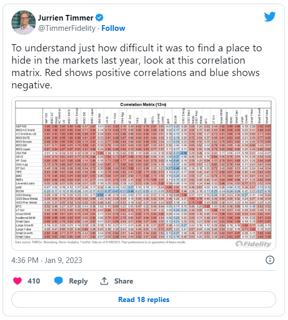
Using this new measure, I propose to compare the diversification potential of the universe of the 11 S&P Sectors in 2021 v.s. in 2022, which was an annus horribilis for diversification as recently quantified by Jurrien Timmer, director of Global Macro at Fidelity, in the tweet reproduced in Figure 5.
In addition to $\frac{1}{DR \left( w_{MDP} \right)^2}$, I also include two other measures of the diversification of a universe of assets:
| Measure | 2021 | 2022 | Comment |
|---|---|---|---|
| $\frac{1}{DR \left( w_{MDP} \right)^2}$ | ~0.42 | ~0.55 | Increase is bad |
| Effective rank | ~4.63 | ~3.27 | Decrease is bad |
| Absorption ratio | ~0.82 | ~0.88 | Increase is bad |
All these measures are unanimous31 in confirming that in 2022, diversification evaporated32!
Examples of usage of the diversification ratio in portfolio optimization
Computation of the most diversified portfolio
Illustration of the core property of the most diversified portfolio
Ref. Property 2, the sorted correlation spectrum of the most diversified portfolio is in theory separated in two distinct regions:
- A region in which correlations are flat, corresponding to the assets with a non-null weight in that portfolio
- A region in which correlations are non-decreasing33, corresponding to the assets with a null weight in that portfolio
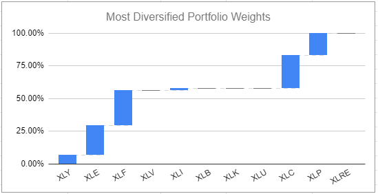
To illustrate how this core property is verified in practice, Figure 6 displays the asset weights of the most diversified portfolio invested in the universe of the 11 S&P Sectors, and Figure 7 displays its sorted correlation spectrum.
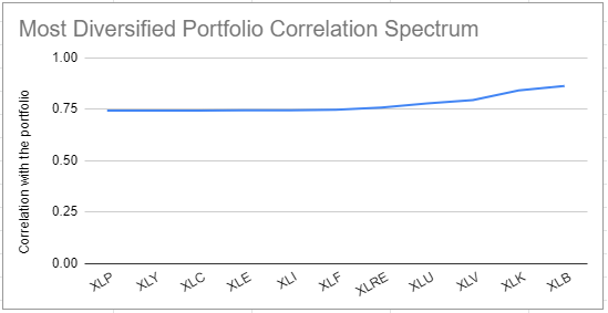
Both theoretical regions are clearly visible in Figure 7 and behave as expected:
- The theoretical flat region is numerically flat34, and contains all the assets with a non-null weight (XLF, XLP, XLC, XLE, XLY, XLI)
- The theoretical non-decreasing region is properly non-decreasing, and contains all the assets with a null weight (XLRE, XLU, XLV, XLK, XLB)
Backtested performance analysis
Backtested performances of the most diversified portfolio have been analyzed within several different universes of assets:
- Within both the universe of the Eurozone equities and the universe of the U.S. equities, by Choueifaty and Coignard1, who find that
most diversified portfolios have higher Sharpe ratios than the market cap–weighted indices and have had both lower volatilities and higher returns in the long run, which can be interpreted as capturing a bigger part of the risk premium
- Within the universe of the MSCI World equities, by Choueifaty et al.2, who conclude that
the [most diversified portfolio] delivers the highest alpha35 of the five strategies tested […] which is consistent with the [most diversified portfolio]’s goal of delivering maximum diversification, and thus a balanced exposure to the effective risk factors available in the universe
- Within the universe of large-cap U.S. stocks, by In Clarke et al.13, who comment
Although high average returns are not the explicit goal of risk-based portfolio construction, all three risk-based portfolios outperform the excess market return
- Within a universe of multiple asset classes (bonds, gold, U.S. equities), by Theron and Van Vuuren36, who summarize in their abstract that
Although previous work has shown that [most diversified] portfolios exhibit greater diversification and a higher Sharpe ratio than other investment strategies, this was not found using developed market index data
Nevertheless, this last paper also states, re-assuringly, that
During the early stages following the financial crisis, the [most diversified] portfolio had the highest, albeit negative, Sharpe ratio […]. This gives us an indication that during this disastrous financial period the [most diversified] portfolio could negate many of the exogenous shocks which impacted the market at that time.
And anyway, it remains to be seen what would have been the conclusion of this paper under a fair comparison of all the tested portfolio allocation methods, because the authors explain that the [most diversified] portfolio was calculated differently to the other three asset allocation portfolios included in the analysis…
So, all in all, backtested performances generally highlight that the most diversified portfolio outperform a market capitalization-weighted portfolio.
Now, what about real-life performances?
Live performance analysis
Thanks to TOBAM, it is possible to go beyond backtested performances of the most diversified portfolio and analyze its real-life performances!
Indeed, the concept of maximum diversification as a portfolio allocation strategy has been patented by TOBAM37, and has been implemented for several years through their suite of Anti-Benchmark funds.
Without further ado, Figure 8, reproduced from Quantalys, shows the live performances over the past three years of the TOBAM Anti-Benchmark US fund38, which is an implementation of the most diversified portfolio within the universe of large and mid-cap U.S. equities.
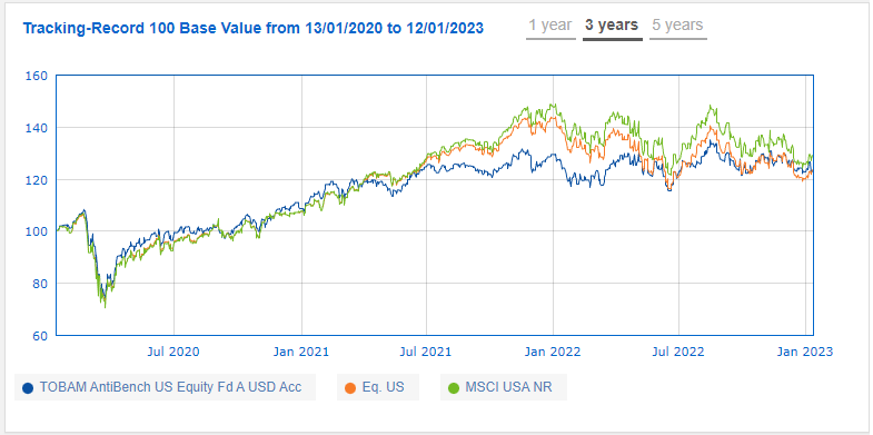
Over that period, the performances of the TOBAM Anti-Benchmark US fund have been comparable to those of the S&P 500, but:
- This fund was not as exposed to the July 2021 - January 2022 market increase as the S&P 500, which might be important for some investors
- This fund was not as exposed to the January 2022 - December 2022 market decrease as the S&P 500, which might be important for other investors
Unfortunately, since inception (not shown in Figure 8), the performances of the TOBAM Anti-Benchmark US fund have been far worse than those of the S&P 500, which would tend to moderate the theoretical claims of over-performance of the most diversified portfolio v.s. a market capitalization-weighted portfolio39.
Diversifying a benchmark portfolio
Through the usage of minimum and maximum asset weight constraints40, the constrained most diversified portfolio can be used to improve the diversification of a benchmark portfolio, for example a market capitalization-weighted portfolio.
For example, Figure 9 displays together:
- The asset weights of the portfolio $P_{SPY}$
- The asset weights of the most diversified portfolio $P_{CMDPSPY}$ constrained to have asset weights within +/- 5% of the asset weights of the $P_{SPY}$ portfolio
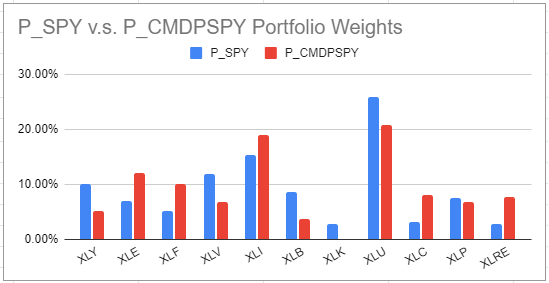
While there is little change in asset weights between these two portfolios, this change is sufficient to boost the diversification ratio of the portfolio representing the S&P 500 by ~6% and the available diversification used by that portfolio by ~9 percentage points41.
| Portfolio | Diversification ratio |
|---|---|
| $P_{SPY}$ | ~1.15 |
| $P_{CMDPSPY}$ | ~1.22 |
| Portfolio | Portfolio squared diversification ratio | MDP squared diversification ratio | Available diversification used by the portfolio | Available diversification not used by the portfolio |
|---|---|---|---|---|
| $P_{SPY}$ | ~1.33 | ~1.81 | ~74% | ~26% |
| $P_{CMDPSPY}$ | ~1.50 | ~1.81 | ~83% | ~17% |
Another possibility to diversify a benchmark portfolio could also be to integrate the diversification ratio as an additional constraint in the benchmark portfolio allocation procedure, but I will not explore this path here.
Conclusion
I hope this first post of 2023 raised your interest in the diversification ratio and in what people at TOBAM are doing re. quantitative investing!
I also hope this post might serve as a motivation to study other uses of the diversification ratio (ex., correlation-based benchmark performance analysis28) as well as of the most diversified portfolio (ex., potential substitute for the diversified risk parity portfolio of Lohre et al.42, which maximizes the effective number of bets within a universe of assets) that I could not detail.
A last word, taken from Clarke et al.13, which I think summarizes particularly well the philosophy behind the diversification ratio:
Some investors traditionally view more securities […] as equivalent to better diversification and lower risk. However, the relatively low number of securities in the maximum diversification […] portfolio[s] illustrate that risk reduction is best achieved by selecting fewer, less correlated and less risky securities, rather than just adding more securities.
As usual, feel free to connect with me on LinkedIn or follow me on Twitter to discuss about Portfolio Optimizer or quantitative finance in general.
–
-
See Choueifaty, Y., Coignard, Y. (2008). Toward maximum diversification. The Journal of Portfolio Management, 35(1), 40–51. ↩ ↩2 ↩3 ↩4 ↩5 ↩6 ↩7
-
See Choueifaty, Y., Tristan Froidure, T., Reynier, J. Properties of the Most Diversified Portfolio. Journal of Investment Strategies, Vol.2(2), Spring 2013, pp.49-70. ↩ ↩2 ↩3 ↩4 ↩5 ↩6 ↩7 ↩8 ↩9 ↩10
-
See Tristan Froidure, Khalid Jalalzai, Yves Choueifaty, Portfolio Rho-Representativity, International Journal of Theoretical and Applied Finance, Vol. 22, No. 07, 1950034 (2019). ↩ ↩2 ↩3 ↩4 ↩5 ↩6 ↩7 ↩8
-
As a reminder, there is no definite formula for diversification, c.f. Meucci43. ↩ ↩2
-
If the covariance matrix is positive semi-definite and not positive definite, these two portfolios might not be unique anymore but all (long-short) most diversified portfolios maximizes the diversification ratio. An interesting question is then how do the different (long-short) most diversified portfolios compare, for example in terms of performance. This question is studied empirically in the case of the most diversified portfolio, in Choueifaty et al.1. ↩
-
For example, if $S$ is a non-empty compact convex set. ↩
-
A risk-based portfolio construction method is a portfolio construction method that does not rely on expected asset returns and requires only expected asset volatilities and correlations. ↩
-
See Wai Lee, Risk-Based Asset Allocation: A New Answer to an Old Question?, The Journal of Portfolio Management Summer 2011, 37 (4) 11-28. ↩ ↩2
-
The constrained most diversified portfolio also satisfy a core property3 in case the constraint set $S$ consists of only the full investment constraint $\sum_{i=1}^{n} w_i = 1$, the non-negativity constraint $w_i \geq 0, i=1..n$ and a common maximum weight constraint $w_i \leq \frac{1}{r}, r \ge 1, i=1..n$. ↩
-
A long-only factor is a factor replicable by long-only portfolios of assets belonging to the universe of assets, c.f. Froidure et al.3. ↩
-
The stability of the most diversified portfolio has also been empirically demonstrated to be better than that of both the equal-risk contributions portfolio and the minimum-variance portfolio in du Plessis and van Rensburg44. ↩
-
See Roger Clarke, Harindra de Silva and Steven Thorley. Risk Parity, Maximum Diversification, and Minimum Variance: An Analytic Perspective. The Journal of Portfolio Management Spring 2013, 39 (3) 39-53. ↩ ↩2 ↩3
-
Under a single-factor risk model, an asset is included in the most diversified portfolio if and only if its correlation with the common factor is lower than a threshold correlation, whose construction tends to eliminates most of the assets in a universe of assets, c.f. Clarke et al.13 ↩
-
See Carmichael, Benoit, Koumou, Nettey Boevi Gilles and Moran, Kevin, (2015), A New Formulation of Maximum Diversification Indexation Using Rao’s Quadratic Entropy, Cahiers de recherche, CIRPEE. ↩
-
Rao’s quadratic entropy is a measure of diversity initially introduced in biology, c.f. Rao45. ↩
-
Choueifaty and Coignard1 and others (Clarke et al.13…) note that the most diversified portfolio is the portfolio with the highest Sharpe ratio if risk is homogeneously proportional to return across the universe of assets, so that the investment problem that the most diversified portfolio solves is compatible with the mean-variance framework. ↩
-
The correlation of the arithmetic returns of the two portfolios is ~0.86. ↩
-
A kind of similar-but-different notion, maximal rho-representativity, is defined and studied in Froidure et al.3. I will not discuss it in this blog post, but several properties of the most diversified portfolio are simply a consequence of it being maximally rho-representative. ↩
-
C.f. Froidure et al.3 for the general methodology. Portfolio Optimizer implements a proprietary variation of that methodology which allows to compute the diversification ratio from time series in most pathological situations. ↩
-
Although counterintuitive, the diversification ratio of the diversified near-minimum variance portfolio might have been lower than the diversification ratio of the minimum variance portfolio in case the additional assets would have increased the average correlation between assets more than they would have decreased the concentration in asset weights. ↩
-
See Meucci, Attilio, Managing Diversification (April 1, 2010). Risk, pp. 74-79, May 2009, Bloomberg Education & Quantitative Research and Education Paper. ↩
-
Using the convention that one year equals 252 daily observations. ↩
-
C.f. the associated blog post for the definitions. ↩
-
The asset weights of the portfolio $P_{SPY}$ in the 11 Sector SPDR ETFs have been set to the reported SPY ETF 11 S&P Sector weights as of beg. January 2023, and using these weights, it is possible to reproduce the evolution of the SPY ETF almost perfectly, which validates this back-of-the-envelope approach. ↩
-
The effective number of bets does not suffer from this issue, because it is bounded by the number of assets. ↩
-
Or, as written in misc. TOBAM Diversification Dashboard reports, how much diversification is left on the table. ↩
-
This typically happens when highly negatively correlated assets are present in a universe of assets, but can also happen due to the asset covariance matrix being (numerically) positive semi-definite and not positive definite. ↩
-
Ref. the observations from Choueifaty et al.2 mentioned previously in this blog post. ↩ ↩2
-
Although again counterintuitive21, $\frac{1}{DR \left( w_{MDP} \right)^2}$ might have been higher in 2022 than in 2021 because the overall increase in correlations could have been counterbalanced by the most diversified portfolio. ↩
-
Nevertheless, c.f. TOBAM’s report Stability of the Pairwise Correlations Hierarchy for explanations on why being well-diversified during market crises remains critical. ↩
-
Or non-increasing, depending on the order of the sort, which is implicitly assumed to be a sort by increasing correlation. ↩
-
Correlations are not exactly equal to $\frac{1}{DR \left( w_{MDP} \right) }$, but are numerically very close, within a +/- 0.3% band. ↩
-
Both Choueifaty and Coignard1 and Choueifaty et al.2 find that the most diversified portfolio provides significant alpha under a three-factor Fama–French model. For why alpha under such a model is important, c.f. for example the podcast snippet Flirting with Models - Vivek Viswanathan, Quant Equity in China - Why Is the Fama-French Three Factor Alpha So Important?. ↩
-
See Theron, Ludan; Van Vuuren, Gary (2018) : The maximum diversification investment strategy: A portfolio performance comparison, Cogent Economics & Finance, ISSN 2332-2039, Taylor & Francis, Abingdon, Vol. 6, Iss. 1, pp. 1-16. ↩
-
See Choueifaty, Y. (2006). Methods and systems for providing an anti-benchmark portfolio. Patent number: USPTO 60/816, 276. ↩
-
Whose ISIN is LU1067856606. ↩
-
All hope is not lost, though, because the TOBAM Anti-Benchmark US fund is not a pure implementation of the most diversified portfolio. Indeed, as can be read from its prospectus, it is subject to many constraints, for example the concentration constraints inherited from its UCITS status. ↩
-
Or other constraints, like a tracking error constraint, which is implemented at TOBAM in their suite of Diversified Benchmark indices. ↩
-
Or ~13%. ↩
-
See Lohre, Harald and Opfer, Heiko and Orszag, Gabor, Diversifying Risk Parity (November 7, 2013). Journal of Risk, Vol. 16, No. 5, 2014, pp. 53-79. ↩
-
See Meucci, Attilio, Managing Diversification (April 1, 2010). Risk, pp. 74-79, May 2009, Bloomberg Education & Quantitative Research and Education Paper. ↩
-
See Hannes du Plessis & Paul van Rensburg (2020): Risk-based portfolio sensitivity to covariance estimation, Investment Analysts Journal. ↩
-
See C.Radhakrishna Rao, Diversity and dissimilarity coefficients: A unified approach, Theoretical Population Biology, Volume 21, Issue 1, 1982, Pages 24-43. ↩