Hierarchical Risk Parity: Introducing Graph Theory and Machine Learning in Portfolio Optimizer
In this short post, I will introduce the Hierarchical Risk Parity portfolio optimization algorithm, initially described by Marcos Lopez de Prado1, and recently implemented in Portfolio Optimizer.
I will not go into the details of this algorithm, though, but simply describe some of its general ideas together with their associated implementation tweaks in Portfolio Optimizer.
Hierarchical risk parity algorithm overview
Step 1 - Hierarchical clustering of the assets
The first step of the Hierarchical Risk Parity algorithm consists in using a hierarchical clustering algorithm to group similar assets together based on their pairwise correlations.
In the original paper, a single linkage clustering algorithm is used1.
In Portfolio Optimizer, 4 hierarchical clustering algorithms are supported:
- (Default) Single linkage
- Complete linkage
- Average linkage
- Ward’s linkage
A good summary of the pros and cons of each of these algorithms can be found in the dissertation of Jochen Papenbrock2.
That being said, practical performances is what ultimately matters, and there seem to be no agreement in the literature nor in the industry about which algorithm to choose.
For example, the performances of the Hierarchical Risk Parity algorithm are reported as deteriorating when single linkage is NOT used3, but Ward’s linkage is used in the computation of the institutional index FIVE Robust Multi-Asset Index…
Anyway, as an illustration of this first step, the following assets correlation matrix taken from a Munich Re4 research note:
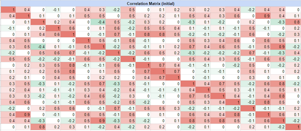
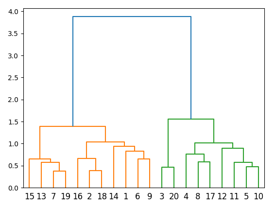
is transformed into the following hierarchical clustering tree, visualized as a dendrogram:
Step 2 - Quasi-diagonalization of the assets correlation matrix
The second step of the Hierarchical Risk Parity algorithm consists in reordering the rows and the columns of the assets correlation matrix according to the order of the leaves of the hierarchical clustering tree computed in the first step5.
Because similar assets are grouped together in the first step, this permutation of the assets correlation matrix tends to reveal a block diagonal structure, hence the name of this second step.
One possible problem with this step is that the order of the leaves of a hierarchical clustering tree is not unique.
Worse, for $n$ assets, there are actually $2^{n-1}$ such orders6!
In Portfolio Optimizer, 2 leaf ordering methods are supported:
- (Default) Leaf ordering following clusters heights, identical to what is implemented in the R function hclust
- Leaf ordering minimizing the distance between adjacent leaves6
The second method is the most appropriate w.r.t. the aim of this second step, but has a running time of one or two orders of magnitude higher than the computation of the hierarchical clustering tree itself, which makes it very costly!
For a small universe of assets ($n \leq 100$), though, the impact on performances is minimal.
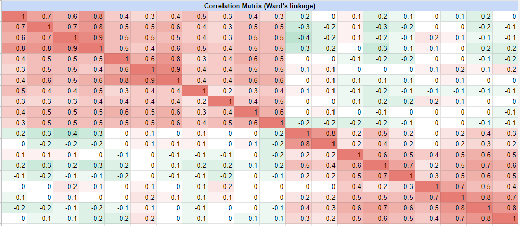
As an illustration of this second step, the assets correlation matrix of Figure 1 becomes, with the default leaf ordering method:
and becomes, with the optimal leaf ordering method:
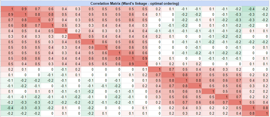
In both Figure 3 and Figure 4, the block diagonal structure hidden in the initial assets correlation matrix now clearly appears.
Step 3 - Recursive bisection and assets weights computation
The third step of the Hierarchical Risk Parity algorithm consists in recursively bisecting the reordered assets correlation matrix computed in the second step and computing assets weights in inverse proportion to both their variance and their clusters variance.
In the original paper, Marcos Lopez de Prado suggests that constraints on assets weights might be incorporated to this step1.
This is what is done in Portfolio Optimizer, which supports minimum and maximum assets weights constraints7 thanks to a variation of the method described in Pfitzinger and Katzke8.
Hierarchical risk parity algorithm usage with Portfolio Optimizer
As a quick practical example of Portfolio Optimizer usage, I propose to reproduce the example provided as Python code in the original paper1.
For this, it suffices to call the Portfolio Optimizer endpoint /portfolios/optimization/hierarchical-risk-parity with the following input data:
This results in the following output, which matches with the expected assets weights9:
{
  "assetsWeights": [0.06999366422693354, 0.07592150585740284, 0.10838947598985076, 0.19029103653662804, 0.09719886787191244, 0.10191545037929818, 0.06618867657198627, 0.09095933462021928, 0.07123881246563615, 0.1279031754801325]
}
Last words
I hope that you will find this new portfolio optimization algorithm useful.
As usual, feel free to reach out if you need any algorithm to be implemented, or if you would like support in integrating Portfolio Optimizer!
–
-
See Lopez de Prado, M. (2016). Building diversified portfolios that outperform out-of-sample. Journal of Portfolio Management, 42(4), 59–69. ↩ ↩2 ↩3 ↩4
-
See Papenbrock, Jochen, Asset Clusters and Asset Networks in Financial Risk Management and Portfolio Optimization. ↩
-
See Thomas Raffinot, The Hierarchical Equal Risk Contribution Portfolio. ↩
-
See Markus Jaeger, Stephan Krugel, Towards robust portfolios, Hierarchical risk parity: persistent diversification uncovered by graph theory and machine learning. ↩
-
Such a procedure is called matrix seriation. ↩
-
See Ziv Bar-Joseph, David K. Gifford, Tommi S. Jaakkola, Fast optimal leaf ordering for hierarchical clustering, Bioinformatics, Volume 17, Issue suppl_1, June 2001, Pages S22–S29. ↩ ↩2
-
This is in contrast to some other closed-source implementations of the Hierarchical Risk Parity algorithm, in which such constraints are managed by a post-process. ↩
-
See Johann Pfitzinger & Nico Katzke, 2019. A constrained hierarchical risk parity algorithm with cluster-based capital allocation. Working Papers 14/2019, Stellenbosch University, Department of Economics. ↩
-
Adaptations to the Python code provided in the original paper1 are required in order to execute it in Python 3, and the computed covariance matrix is not the same between Python 2 and Python 3! ↩