Computation of Theory-Implied Correlation Matrices: Overview and Example

7 minute read

In this short post, I will provide an overview of the TIC algorithm¹ introduced by Marcos Lopez de Prado in his paper Estimation of Theory-Implied Correlation Matrices², which aims to compute a forward-looking asset correlation matrix blending both empirical and theoretical inputs.

I will also describe the associated implementation tweaks in Portfolio Optimizer.

Notes:

A Google sheet corresponding to this post is available here

Theory-Implied Correlation algorithm overview

Step 1 - Constrained hierarchical clustering of the assets

The first step of the Theory-Implied Correlation algorithm consists in using a hierarchical clustering algorithm to group similar assets together based on a distance metric $d$ derived from their pairwise correlations, defined as

\[d_{i,j} = \sqrt{\frac{1}{2} (1 - c_{i,j})}\]

where $d_{i,j}$ (resp. $c_{i,j}$) is the distance (resp. the correlation) between asset $i$ and asset $j$, $i,j = 1..n$, with $n \ge 2$ the total number of assets.

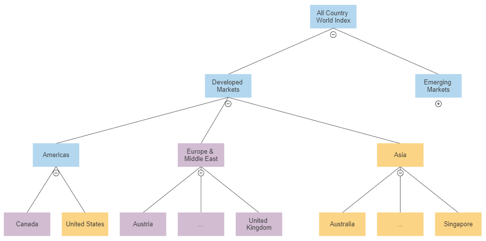
Nevertheless, and contrary for example to the Hierarchical Risk parity algorithm, the hierarchical clustering algorithm is constrained to match a prior represented by a theoretical tree graph structure, which usually corresponds to a hierarchical classification of the assets like:

The Standard Industrial Classification or the MSCI Global Industry Classification Standard when assets are stocks
The MSCI ACWI Index market allocation, illustrated in Figure 1, when assets are country ETFs

Figure 1. MSCI ACWI Index market allocation as a hierarchical classification.

The result of this first step is a hierarchical clustering tree which somewhat best matches the asset correlations with the theoretical tree structure³.

In the code accompanying the original paper², a combination of a single linkage clustering algorithm⁴ and of a custom average linkage clustering algorithm⁵ is used as the hierarchical clustering algorithm.

In Portfolio Optimizer, 4 hierarchical clustering algorithms are supported⁶:

Single linkage
Complete linkage
(Default) Average linkage
Ward’s linkage

Also, in Portfolio Optimizer, the number of levels of the theoretical tree graph structure is limited to 4, which corresponds to the 4 levels of the MSCI GICS hierarchical classification⁷.

Step 2 - Computation of the implied asset correlation matrix

The second step of the Theory-Implied Correlation algorithm consists in determining the asset correlation matrix associated with the hierarchical clustering tree computed in the first step.

This is done by inverting the relationship between the distance metric $d$ and the assets correlation $c_{i,j}$, $i,j = 1..n$, which leads to

\[c_{i,j} = 1 - 2 d_{C_i, C_j}^2\]

where $C_i$ and $C_j$ are the two clusters of the hierarchical clustering tree satisfying the following properties:

$C_i$ and $C_j$ are the two children of a node $n$ of the hierarchical clustering tree such that asset $i$ belongs to $C_i$ and asset $j$ belongs to $C_j$
There are no other clusters $\hat{C}_i$ and $\hat{C}_j$ that are the two children of a node $\hat{n}$, indirect child of the node $n$, such that asset $i$ belongs to $\hat{C}_i$ and asset $j$ belongs to $\hat{C}_j$

In other words, $C_i$ and $C_j$ are the two children of the deepest node $n$ of the hierarchical clustering tree such that asset $i$ belongs to $C_i$ and asset $j$ belongs to $C_j$.

Step 3 - De-noising of the implied asset correlation matrix

The third and final step of the Theory-Implied Correlation algorithm consists in altering the implied asset correlation matrix computed in the second step to transform it into a valid correlation matrix.

Indeed, as noted by Marcos Lopez de Prado²:

The correlation matrix derived from the [hierarchical clustering tree] may not be definite positive, or it may have a high condition number.

In the code accompanying the original paper², the implied asset correlation matrix is denoised using an algorithm based on random matrix theory and detailed by Marcos Lopez de Prado in his book Machine Learning for Asset Managers⁸.

Personally, I find that denoising the initial asset correlation matrix - as opposed to the implied asset correlation matrix - makes more sense theoretically.

That’s why in Portfolio Optimizer such an alteration of the implied asset correlation matrix is left to the user and would anyway rather be performed by calling one of the following API endpoints:

/assets/correlation/matrix/nearest, to compute the nearest correlation matrix from the implied asset correlation matrix

Theory-Implied Correlation algorithm usage with Portfolio Optimizer

As a quick practical example of Portfolio Optimizer usage, I will reproduce the example from the article of Hudson & Thames Portfolio Optimisation with PortfolioLab: Theory-Implied Correlation Matrix.

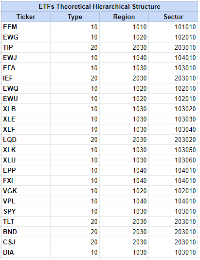
In order to illustrate their own TIC algorithm, Hudson & Thames propose to work with a universe of 23 ETFs⁹ for which they define the theoretical tree graph structure displayed in Figure 2.

Figure 2. Theoretical tree graph structure of the Hudson & Thames universe of 23 ETFs.

Thanks to their PortfolioLab Python library, they compute the de-noised theory-implied correlation matrix of these 23 ETFs and they compare it to the original empirical correlation matrix of these same 23 ETFs.

I will do the same with Portfolio Optimizer.

Computation of the ETFs empirical correlation matrix

Thanks to price data retrieved from both¹⁰ Tiingo and Alpha Vantage, as well as to the Portfolio Optimizer API endpoints
/assets/returns and /assets/correlation/matrix, the empirical correlation matrix of the 23 ETFs is immediate to compute and is illustrated in Figure 3.

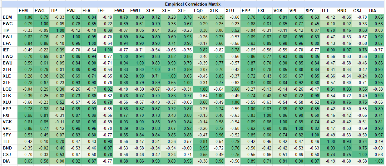
Figure 3. Empirical correlation matrix of the Hudson & Thames universe of 23 ETFs.

This empirical correlation matrix is nearly perfectly matching the empirical correlation matrix from Hudson & Thames, except for the XLU ETF which exhibit a negative correlation to the equity ETFs and a positive correlation to the bonds ETFs over the selected period!

Computation of the raw ETFs theory-implied correlation matrix

Using the computed empirical correlation matrix together with the theoretical tree graph structure displayed in Figure 2, it is possible to compute the raw, non de-noised, theory-implied correlation matrix of the 23 ETFs.

With Portfolio Optimizer, this is done through the following invocation of the API endpoint /assets/correlation/matrix/theory-implied

    
	fetch('https://api.portfoliooptimizer.io/v1/assets/correlation/matrix/theory-implied', 
	      { 
		    method: 'POST',
		    headers: { 'Content-Type': 'application/json' },
            body: JSON.stringify({ assets: [ {assetHierarchicalClassification: [10, 1010, 101010]}, ... ],
                                   assetsCorrelationMatrix: [[1.0,0.7943899971154988, ...], ...]
                                 }) 
          })

, which returns

       
{
   "assetsCorrelationMatrix":[[1,0.8129900881613477, ...], ...]
}

This correlation matrix is unfortunately not positive semi-definite¹¹, so that it needs to be transformed into a valid correlation matrix.

Computation of the final ETFs theory-implied correlation matrix

As mentioned earlier in this post, “fixing” a non positive semi-definite theory-implied correlation matrix can be done with the Portfolio Optimizer API endpoint /assets/correlation/matrix/nearest.

Here, the resulting valid theory-implied correlation matrix is illustrated in Figure 4.

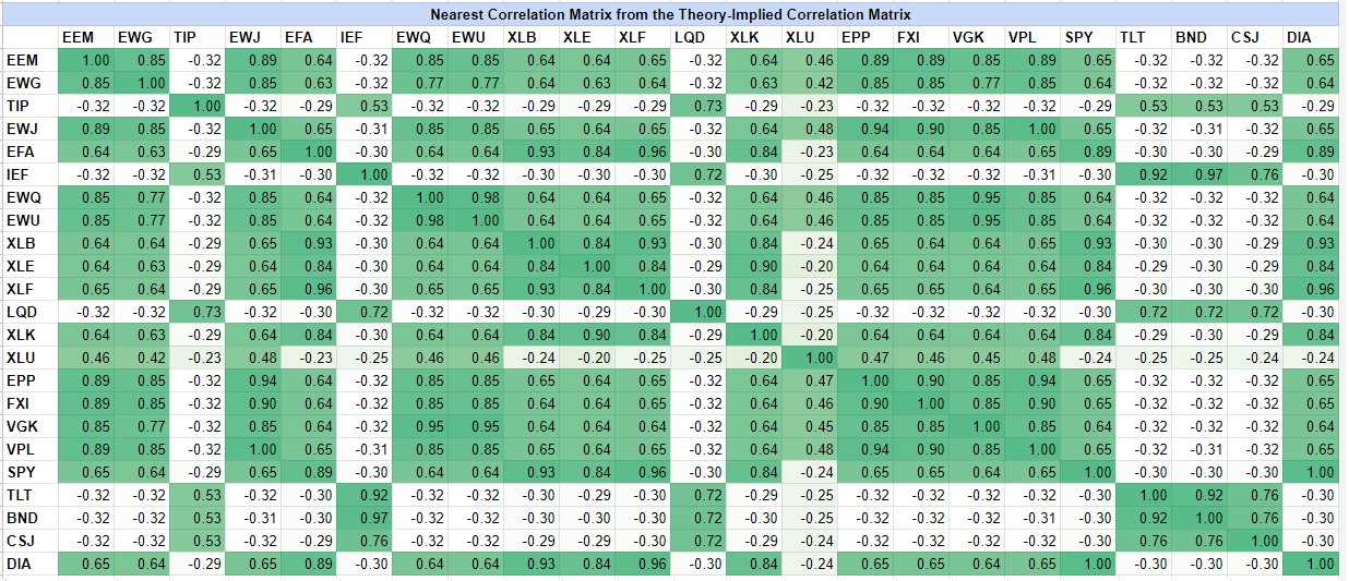
Figure 4. Nearest correlation matrix from the theory-implied correlation matrix of the Hudson & Thames universe of 23 ETFs.

Again, this final theory-implied correlation matrix is nearly perfectly matching its equivalent from Hudson & Thames, except for the XLU ETF.

Computation of the distance from the ETFs empirical correlation matrix to the final ETFs theory-implied correlation matrix

As a last step, it is possible to compute the distance from the ETFs empirical correlation matrix to the final ETFs theory-implied correlation matrix.

For this, and like both in the paper from Marcos Lopez de Prado² and in the article from Hudson & Thames, I will use a distance called the correlation matrix distance¹² implemented in Portfolio Optimizer API endpoint /assets/correlation/matrix/distance.

The computed distance is $\approx 0.105$, which is much greater than the computed distance of $\approx 0.036$ in the article from Hudson & Thames, but since the correlation data for the XLU ETF completely differs, this is not unexpected.

In any cases, this distance is of the same order of magnitude as the distance computed by Marcos Lopez de Prado for the S&P 500², so that, as he puts it:

While [the] TIC [matrix] departs from the empirical correlation matrix […], the two are not too far apart. This corroborates that the TIC matrix has blended theory-implied views with empirical evidence.

Last words

No specific last words this time, except that I recently created my LinkedIn profile.

So, feel free to connect with me to discuss about Portfolio Optimizer or more generally quantitative stuff!

–

TIC algorithm stands for Theory-Implied Correlation algorithm. ↩
See Lopez de Prado, Marcos Estimation of Theory-Implied Correlation Matrices (November 9, 2019). ↩ ↩² ↩³ ↩⁴ ↩⁵ ↩⁶
For example, in case of a universe of assets made of the country ETFs illustrated on Figure 1, an unconstrained hierarchical clustering algorithm might cluster together the Canada ETF and the Singapore ETF, while the Theory-Implied Correlation algorithm will always first cluster together the Canada ETF and the United States ETF on one hand and all the Asia region ETFs on the other hand. ↩
Used to cluster the leaves of the theoretical tree graph structure. ↩
Used to compute the distances between newly created clusters and old clusters. ↩
Used both to cluster the leaves of the theoretical tree graph structure AND to compute the distances between newly created clusters and old clusters, so that contrary to the original paper², there is a unique hierarchical clustering algorithm used throughout all the process. ↩
This limit is neither a technical limit nor an API limit, so that it can be increased - if ever needed - by simply reaching out. ↩
See Lopez de Prado, M. (2019): Machine Learning for Asset Managers. Cambridge University Press, First edition. ↩
The 23 ETFs are EEM, EWG, TIP, EWJ, EFA, IEF, EWQ, EWU, XLB, XLE, XLF, LQD, XLK, XLU, EPP, FXI, VGK, VPL, SPY, TLT, BND, CSJ, DIA. ↩
Price data have been retrieved from Tiingo for all the ETFs except CSJ and from Alpha Vantage for CSJ and are covering the period 2017-07-31 to 2018-07-31. This latter date corresponds to the termination date of the CSJ ETF. ↩
This can be verified thanks to the Portfolio Optimizer API endpoint /assets/correlation/matrix/validation. ↩
See M. Herdin, N. Czink, H. Ozcelik and E. Bonek, “Correlation matrix distance, a meaningful measure for evaluation of non-stationary MIMO channels,” 2005 IEEE 61st Vehicular Technology Conference, 2005, pp. 136-140 Vol. 1, doi: 10.1109/VETECS.2005.1543265. ↩