Correlation Matrix Stress Testing: Shrinkage Toward an Equicorrelation Matrix

Financial research has consistently shown that correlations between assets tend to increase during crises and tend to decrease during recoveries¹.

The recent COVID-19 market crash was no exception, as illustrated on Alvarez Quant Trading blog post Correlations go to One for both the individual constituents of the S&P500 and several broad ETFs commonly used in tactical asset allocation strategies.

From a portfolio management perspective, this implies that it is important to understand the impact of sudden changes in correlations before they materialize.

One way to proceed is to alter a baseline correlation matrix by incorporating extreme correlation changes in its coefficients and evaluate how this altered correlation matrix translates into a different portfolio allocation², a higher portfolio Value at Risk³, etc.

This procedure is usually called correlation (matrix) stress testing.

However, this altered correlation matrix may become invalid⁴ and not usable anymore in numerical algorithms!

In a previous post, I mentioned that such an invalid correlation matrix could be fixed thanks to the nearest correlation matrix algorithm, as implemented for example in Portfolio Optimizer.

In this post, I will introduce another method, maybe more intuitive, which relies on the shrinkage of the baseline correlation matrix toward an equicorrelation matrix representing the desired crisis state.

Notes:

• A fully functional Google sheet corresponding to this post is available here
• Main references for this post are two papers: one from Andreas Steiner⁵ and one from Kawee Numpacharoen⁶, in which the shrinkage method is called the Weighted Average Correlation Matrices method

Mathematical preliminaries

Equicorrelation matrices

An equicorrelation matrix of order $n \geq 2$ is a matrix $C_{\rho} \in \mathcal{M} \left( \mathbb{R}^{n \times n} \right)$ which:

• Is unit diagonal: $(C_{\rho})_{i,i} = 1$, $i=1..n$
• Is symmetric and has all its off-diagonal coefficients equal to a common parameter $\rho \in [-1,1]$: $(C_{\rho})_{i,j} = \rho$, $i,j=1..n, i \ne j$
• Is positive semi-definite

In other words, \(C_{\rho} = \begin{pmatrix} 1 & \rho & \rho & \dots & \rho \\ \rho & 1 & \rho & \dots & \rho \\ \vdots & \vdots & \vdots & \ddots & \vdots \\ \rho & \rho & \rho &\dots & 1 \end{pmatrix}\) , with $\rho \in [-1,1]$ such that $C_{\rho}$ is positive semi-definite.

One interesting property that can be established is that the matrix $C_{\rho}$ is positive semi-definite if and only if $\rho \in [-\frac{1}{n-1}, 1]$, which unfortunately severely restricts the magnitude of the negative values of the parameter $\rho$, especially in high dimension.

Let’s quickly demonstrate this result.

The matrix $C_{\rho}$ has two eigenvalues⁷:

• $1 + (n-1) \rho$, of multiplicity 1, associated to the eigenvector $u_1 = (1, \dots, 1) {}^t$
• $1 - \rho$, of multiplicity $n-1$⁸, associated to the $n-1$ eigenvectors $u_2, \dots, u_n$, with \((u_k)_i = \begin{cases} 1 &\text{if } i = 1, \\ -1 &\text{if } i = k, \\ 0 &\text{otherwise.} \end{cases}\)

So, because a symmetric matrix is positive semi-definite if and only if all its eigenvalues are non-negative, the matrix $C_{\rho}$ is positive semi-definite if and only if $1 + (n-1) \rho \geq 0$ and $1 - \rho \geq 0$, that is, $\rho \in [-\frac{1}{n-1}, 1]$.

Shrinkage

The usage of shrinkage estimation of covariance (or correlation) matrices in finance was popularized in the 2000s by Olivier Ledoit and Michael Wolf⁹.

The basic idea is to form a convex linear combination of two covariance (or correlation) matrices in order to reach a balance between their properties.

More formally, given

• A reference correlation matrix $C \in \mathcal{M}(\mathbb{R}^{n \times n})$
• A target correlation matrix $T \in \mathcal{M}(\mathbb{R}^{n \times n})$
• A shrinkage factor¹⁰ $\lambda \in [0,1]$

, shrinking the matrix $C$ toward the matrix $T$ is done by computing the matrix \(S_{\lambda} = (1-\lambda) C + \lambda T\).

To be noted that the matrix $S_{\lambda}$ is a valid correlation matrix for any $\lambda \in [0,1]$, because it is easily established that $S_{\lambda}$ is

• Symmetric: $S_{\lambda} {}^t = S_{\lambda}$
• Unit diagonal: $(S_{\lambda})_{i,i} = 1$, $i=1..n$
• Positive semi-definite: $x {}^t S_{\lambda} x \geq 0, x \in \mathbb{R}^{n}$

Correlation matrix stress testing scenarios

The stylized facts of financial crises described in the introduction lead to envisage three (systemic) correlation stress testing scenarios.

Correlations increasing to one

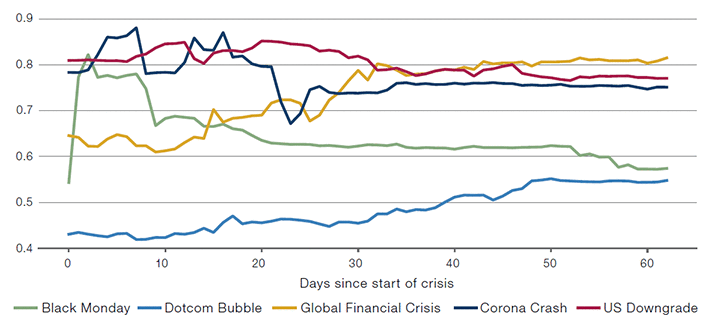
This is the typical scenario for global equities during the onset of a major financial crisis, as illustrated on figure 1 taken from the article Covid Crash Risk — What’s in a Number? of the Man Institute.

Figure 1. Rolling correlations of the S&P500 Index v.s. the EuroStoxx50 Index. Source: Man Institute

This scenario can be simulated through the shrinkage of a baseline correlation matrix toward the equicorrelation matrix \(C_1 = \begin{pmatrix} 1 & 1 & 1 & \dots & 1 \\ 1 & 1 & 1 & \dots & 1 \\ \vdots & \vdots & \vdots & \ddots & \vdots \\ 1 & 1 & 1 &\dots & 1 \end{pmatrix}\), representing a state of maximum correlation.

Correlations decreasing to zero

This scenario is frequently occuring for global equities during the recovery of a major financial crisis, as also illustrated on figure 1 for the Black Monday, the US Downgrade and the Corona Crash crises.

This scenario is also documented to be occuring for some asset classes like bonds¹¹ or in international currency markets¹² during market turbulences.

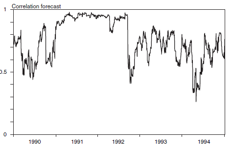
For example, figure 2 taken from Philippe Jorion’s book¹² illustrates the turbulences around the devaluation of the British Pound in September 1992, which would have been devastating for a market-neutral trader long British Pound - short Deutsche Mark.

Figure 2. Rolling correlations of the British Pound v.s. the Deutsche Mark. Source: Philippe Jorion's book

This scenario can be simulated through the shrinkage of a baseline correlation matrix toward the equicorrelation matrix \(C_0 = \begin{pmatrix} 1 & 0 & 0 & \dots & 0 \\ 0 & 1 & 0 & \dots & 0 \\ \vdots & \vdots & \vdots & \ddots & \vdots \\ 0 & 0 & 0 &\dots & 1 \end{pmatrix}\), representing a state of maximum decorrelation.

Correlations decreasing to minus one

This scenario is the mirror of the first one, and is known to be occurring for risk factors of fixed income portfolios¹³ during market distress with aggressive central banks intervention.

Ideally, this scenario could have been simulated through the shrinkage of a baseline correlation matrix toward the matrix \(C_{-1} = \begin{pmatrix} 1 & -1 & -1 & \dots & -1 \\ -1 & 1 & -1 & \dots & -1 \\ \vdots & \vdots & \vdots & \ddots & \vdots \\ -1 & -1 & -1 &\dots & 1 \end{pmatrix}\), representing a state of maximum anticorrelation.

Unfortunately, as demonstrated in the mathematical preliminaries of this post, the matrix $C_{-1}$ is not an equicorrelation matrix because $-1 < -\frac{1}{n-1}$.

So, this scenario can only be partially simulated through the shrinkage of a baseline correlation matrix toward the equicorrelation matrix \(C_{-\frac{1}{n-1}} = \begin{pmatrix} 1 & -\frac{1}{n-1} & -\frac{1}{n-1} & \dots & -\frac{1}{n-1} \\ -\frac{1}{n-1} & 1 & -\frac{1}{n-1} & \dots & -\frac{1}{n-1} \\ \vdots & \vdots & \vdots & \ddots & \vdots \\ -\frac{1}{n-1} & -\frac{1}{n-1} & -\frac{1}{n-1} &\dots & 1 \end{pmatrix}\), representing a state of maximum achievable anticorrelation.

Determination of the value of the shrinkage factor

For any correlation stress testing scenario simulated through shrinkage, the shrinkage factor $\lambda$ can be interpreted as a way to incorporate the probability of occurrence of the scenario:

• For $\lambda = 0$, $S_{\lambda} = C$, so that the shrunk correlation matrix is equal to the baseline correlation matrix. This can be interpreted as a 0% probability of realization of the stress scenario.
• For $\lambda = 1$, $S_{\lambda} = T$, so that the shrunk correlation matrix is equal to the target equicorrelation matrix. This can be interpreted as a 100% probability of realization of the stress scenario.
• For $\lambda \in ]0,1[$, the shrunk correlation matrix $S_{\lambda}$ is more and more departing from the baseline correlation matrix $C$ and approaching the target correlation matrix $T$ as $\lambda \to 1$. This can be interpreted as a $\lambda$ % probability of realisation of the stress scenario.

So, for example, if the probability of occurrence of a given scenario is evaluated to 50%, the value of the shrinkage factor $\lambda$ could be set to 50%.

Notes:

• The interpretation of the shrinkage factor $\lambda$ as a percentage is described in one of the main references of this post⁶, but is, by definition, rather subjective. A more data-driven procedure to determine this factor is proposed in the next paragraph.

Example of application - Preparing for the next financial crisis

Suppose that we are managing a portfolio of broad ETFs, in the same universe¹⁴ as the J.P. Morgan Efficiente 5 Index.

Suppose also that on 20 August 2021, we would like to assess the impact on our universe of ETFs of a correlations breakdown similar to the one which occurred during the Corona Crash.

What could we do?

Well, because we read this blog post carefully , we would like to compute a stressed correlation matrix $C_{shrunk}$ by shrinking the current asset correlation matrix $C_{current}$ toward the equicorrelation matrix $C_1$, that is

\[C_{shrunk} = (1-\lambda) C_{current} + \lambda C_1\]

with $\lambda \in ]0,1[$ to be determined.

Determination of a data-driven shrinkage factor

Unfortunately, we have no view on the probability of occurrence of a market crash, so that we are unable to choose a subjective shrinkage factor $\lambda$.

One data-driven possibility is then to compute $\lambda$ so that the (Frobenius) distance¹⁵ between the current asset correlation matrix and the stressed correlation matrix is the same as the distance between the pre-Corona Crash asset correlation matrix and the Corona Crash asset correlation matrix.

Formally, we would like

\[d_F(C_{current}, C_{shrunk}) = d_F(C_{pre-Corona \, Crash}, C_{Corona \, Crash})\]

So, given that

\[\begin{aligned} d_F(C_{current}, C_{shrunk}) &= \left\Vert C_{current} - C_{shrunk} \right\Vert_F \\ &= \left\Vert C_{current} - ((1-\lambda) C_{current} + \lambda C_1) \right\Vert_F \\ &= \lambda \left\Vert C_{current} - C_1 \right\Vert_F \\ &= \lambda d_F(C_{current}, C_1)\end{aligned}\]

It implies

\[\lambda = \frac{d_F(C_{pre-Corona \, Crash}, C_{Corona \, Crash})}{d_F(C_{current}, C_1)}\]

Computation of the data-driven shrinkage factor

Let’s first compute $d_F(C_{pre-Corona \, Crash}, C_{Corona \, Crash})$.

For this, we need to define the exact two time periods pre-Corona Crash and Corona Crash:

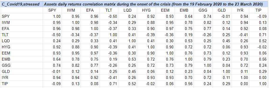
• For the later, I chose the period 19 February 2020 - 23 March 2020, which corresponds to the peak of the financial crisis¹⁶
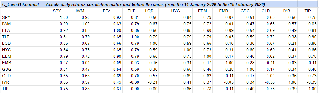
• For the former, I chose the period 14 January 2020 - 18 February 2020, which corresponds to the period preceding the peak of the financial crisis with the same number of trading days

This leads to $C_{pre-Corona \, Crash}$

Figure 3. Daily returns correlation matrix between 12 ETFs over the period 14 January 2020 - 18 February 2020

and to $C_{Corona \, Crash}$¹⁷

Figure 4. Daily returns correlation matrix between 12 ETFs over the period 19 February 2020 - 23 March 2020

so that $d_F(C_{pre-Corona \, Crash}, C_{Corona \, Crash}) \approx 6.03$.

Let’s then compute $d_F(C_{current}, C_1)$, for which I chose to define the current period as the period 20 July 2021 - 20 August 2021¹⁸

Figure 5. Daily returns correlation matrix between 12 ETFs over the period 20 July 2021 to the 20 August 2021

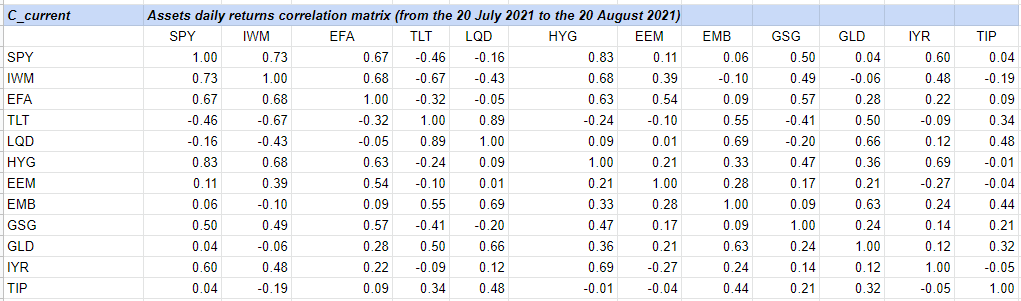
so that $d_F(C_{current}, C_1) \approx 9.84$.

Let’s finally compute the shrinkage factor $\lambda$, that is, $\lambda \approx \frac{6.03}{9.84} \approx 0.61$.

Computation of the stressed correlation matrix

Thanks to the computation of the shrinkage factor, it is now possible to compute the shrunk correlation matrix, for example with the Portfolio Optimizer endpoint /assets/correlation/matrix/shrinkage.

This leads to $C_{shrunk}$

Figure 6. Stressed (shrunk) correlation matrix between 12 ETFs, to prepare for the next crisis

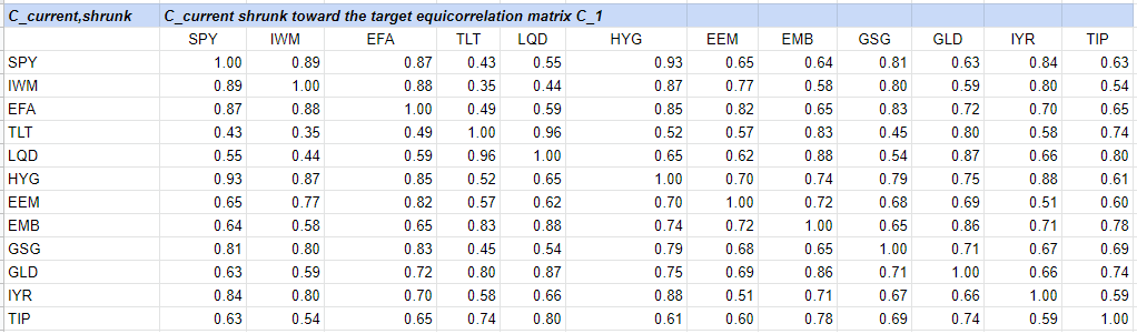
We can notice¹⁹ that the increase in correlations between the matrices $C_{current}$ and $C_{shrunk}$ is comparable to the increase in correlations observed during the Corona Crash between the matrices $C_{pre-Corona \, Crash}$ and $C_{Corona \, Crash}$.

We can also notice one possible issue, which is that correlations are increasing between all the assets, while during the Corona Crash a couple of assets saw their correlations actually decrease, like gold and long term treasuries.

Nevertheless, given that each crisis is usually of different nature, such unexpected changes in correlations might ultimately be desirable!

Conclusion

What to do next with the stressed correlation matrix $C_{shrunk}$ is up to one’s imagination or requirements.

One possibility could be to compute an associated optimal portfolio allocation²⁰ and compare it to the current portfolio allocation. This would help determining the robustness of the current portfolio to extreme correlation changes.

–

1. See Sebastien Page & Robert A. Panariello (2018) When Diversification Fails, Financial Analysts Journal, 74:3, 19-32 and references therein. ↩

2. See Rachel Campbell, Kees Koedijk and Paul Kofman, Increased Correlation in Bear Markets, Financial Analysts Journal Vol. 58, No. 1, pp. 87-94. ↩

3. See Paul H. Kupiec, Stress Testing in a Value at Risk Framework, The Journal of Derivatives Aug 1998, 6 (1) 7-24. ↩

4. Usually, non positive semi-definite. ↩

5. See Steiner, Andreas, Manipulating Valid Correlation Matrices. ↩

6. See Kawee Numpacharoen, Weighted Average Correlation Matrices Method for Correlation Stress Testing and Sensitivity Analysis, The Journal of Derivatives Nov 2013, 21 (2) 67-74. ↩ ↩²

7. This can be verified by using the definition of an eigenvalue. For example, $C_{\rho} u_1 = (1 + (n-1) \rho) u_1$, so that by definition $u_1$ is an eigenvector associated to the eigenvalue $1 + (n-1) \rho$. ↩

8. The eigenvectors $u_2, \dots ,u_n$ are linearly independent, which can easily be verified using the definition of linear independence of a vector set. So, the dimension of the eigenspace associated to the eigenvalue $1 - \rho$ is $n-1$. ↩

9. See Olivier Ledoit and Michael Wolf, Honey, I Shrunk the Sample Covariance Matrix, The Journal of Portfolio Management Summer 2004, 30 (4) 110-119. ↩

10. Also called shrinkage intensity or shrinkage constant. ↩

11. See Mark Kritzman, Kenneth Lowry and Anne-Sophie Van Royen, Risk, Regimes, and Overconfidence, The Journal of Derivatives Spring 2001, 8 (3) 32-42. ↩

12. See Philippe Jorion, Value at Risk: The New Benchmark for Managing Financial Risk, McGraw-Hill Professional; 3rd Revised edition. ↩ ↩²

13. See Bhansali, Vineer and Wise, Mark B., Forecasting Portfolio Risk in Normal and Stressed Markets ↩

14. Excluding the cash-equivalent ETF SGOV, because it would make no sense to increase the correlation of cash to any other asset. ↩

15. See Frobenius norm ↩

16. C.f. Wikipedia, In the 33 days between 19 February and 23 March, […] the MSCI World Index declined by 34 per cent. ↩

17. On which an extreme increase in most correlations is visible. For example, the correlation between the two ETFs LQD and HYG spikes from -0.59 to 0.41! ↩

18. This period is the most current period at the time of preparation of this blog post with the same number of trading days as the peak of the Corona Crash time period. ↩

19. E.g., the correlation between the 2 ETFs SPY and LQD went from -0.56 to 0.24 during the Corona Crash, and increases from -0.16 to 0.55 with the computed stressed correlation matrix. ↩

20. Possibly also revising future assets return and/or assets volatility with a similar methodology. ↩