The Effective Number of Bets: Measuring Portfolio Diversification
Many different measures of portfolio diversification have been developed in the financial literature, from asset weights-based diversification measures like the Herfindahl Index1 to risk-based diversification measures like the diversification ratio of Choueifaty and Coignard2 to other more complex diversification measures.
Because each of these measures usually provides information about a different aspect of a portfolio, they all complement each other.
In this post, I will describe a measure introduced by Attilio Meucci3 and called the effective number of bets, which quantifies the degree of diversification of a portfolio through its exposure to uncorrelated risk factors associated to the assets it contains.
Notes:
- A Google sheet corresponding to this post is available here
Mathematical preliminaries
Let be:
- $n \ge 2$, the number of assets in a universe of assets
- $w \in \mathbb{R}^{n}$, the asset weights of a portfolio in this universe of assets
- $\Sigma \in \mathcal{M}(\mathbb{R}^{n \times n})$, the asset covariance matrix
- $\mathring{l} \in \mathcal{M}(\mathbb{R}^{n \times n})$, an invertible matrix such that $ \mathring{\Sigma} = \mathring{l} \Sigma \mathring{l} {}^t $ is a diagonal matrix
Definitions
Diversification distribution
The diversification distribution $d(w) \in [0,1]^{n}$ of the portfolio with asset weights $w$ is defined as
\[d(w) = \frac{ \left( \left( \mathring{l} {}^t \right)^{-1} w \right) \circ \left( \mathring{l} \Sigma w \right) }{w {}^t \Sigma w}\]where $\circ$ denotes the Hadamard product.
Effective number of bets
The effective number of bets (ENB) $\mathcal{N}_{Ent}(w) \in [1,n]$ of the portfolio with asset weights $w$ is defined as4
\[\mathcal{N}_{Ent}(w) = e^{- \sum_{i=1}^{n} {d(w)}_i \ln {d(w)}_i}\]Rationale
In the traditional risk parity literature, the risk contribution of an asset to a portfolio suffers from the practical shortcoming that it is usually affected by the risk contributions of all the other assets due to their non-null correlations5.
To solve this shortcoming, Meucci et al.6 propose to transform the $n$ original assets into $n$ new uncorrelated synthetic assets7 - or implicit risk factors -
so that it becomes possible to interpret the (percentage) risk contributions of these synthetic assets as a probability distribution of independent events, which
leads to the definition of the diversification distribution.
The matrix $\mathring{l}$8 corresponds to this transformation, with:
- $\mathring{l}_{i,j}$ the weight of the original asset $j=1..n$ in the synthetic asset $i=1..n$
- $\mathring{\Sigma} = \mathring{l} \Sigma \mathring{l} {}^t$ the covariance matrix of the synthetic assets, diagonal as per the listed requirements
Finally, in order to summarize the information contained in the diversification distribution in one single number, Meucci et al.6 define the ENB as its exponential Shannon entropy.
This definition allows the ENB to measure the diversification of a portfolio through its exposure to uncorrelated risk factors associated to the assets it contains.
Properties
The main property of the ENB is that:
- $\mathcal{N}_{Ent}(w) = 1$ if and only if the portfolio with asset weights $w$ is fully concentrated, with an exposure equal to 1 to a unique risk factor
- $\mathcal{N}_{Ent}(w) = n$ if and only if the portfolio with asset weights $w$ is fully diversified, with an exposure equal to $\frac{1}{n}$ to the $n$ risk factors
The decorrelating matrix $\mathring{l}$
In theory, it is possible to choose any matrix $\mathring{l}$ satisfying the listed requirements to compute the ENB9, but the choice of this matrix impacts the properties of the ENB as an intuitive measure of portfolio diversification as illustrated in Meucci et al.6.
Consequently, Meucci3 and Meucci et al.6 recommend to choose either:
- The (transpose of the) matrix of the principal components of the asset covariance matrix $\Sigma$10, that is, $\mathring{l} = e {}^t$ with $e \in \mathcal{M}(\mathbb{R}^{n \times n})$ such that $ \Sigma = e \lambda^2 e {}^t$ where $\lambda \in \mathcal{M}(\mathbb{R}^{n \times n})$ is the diagonal matrix of the singular values of the covariance matrix $\Sigma$
- The minimum linear torsion transformation matrix defined as the matrix representing the linear transformation which decorrelates the asset returns used to compute the asset covariance matrix $\Sigma$ while keeping them as close as possible to their original values, that is, $\mathring{l} = \mathring{t}_{MT}$ c.f. Meucci et al.6
Notes:6
- When the matrix $e {}^t$ is chosen as the decorrelating matrix, the diversification distribution is called the principal components diversification distribution and the effective number of bets is called the effective number of principal components bets
- When the matrix $\mathring{t}_{MT}$ is chosen as the decorrelating matrix, the diversification distribution is called the minimum torsion diversification distribution and the effective number of bets is called the effective number of minimum torsion bets
Effective number of principal component bets
Choosing the matrix $e {}^t$ as the decorrelating matrix has been initially proposed in Meucci3, but later abandoned for several reasons explained in Meucci et al.6 (instability and non-unicity of the principal components…).
The most important of these reasons, also identified by people at Flirting with Models in their blog post Using Simple Examples to Gain Quantitative Insight, is that using the (transpose of the) matrix of the principal components leads to counter-intuitive results.
Indeed, let’s consider as in Meucci et al.6 a universe of $n \geq 2$ assets with equal volatility $\sigma^2$ and equal positive pairwise correlation $\rho > 0$, that is, with a covariance matrix equal to
\[\begin{pmatrix} \sigma^2 & \rho \sigma^2 & \dots & \rho \sigma^2 \\ \rho \sigma^2 & \sigma^2 & \dots & \rho \sigma^2 \\ \vdots & \vdots & \ddots & \vdots \\ \rho \sigma^2 & \rho \sigma^2 & \dots & \sigma^2 \end{pmatrix}\]If the common correlation factor $\rho$ is taken approximately null, the equal-weighted portfolio $w_{EW} = (\frac{1}{n},…,\frac{1}{n})$ is then fully diversified w.r.t. $n$ nearly uncorrelated assets.
By definition, its associated effective number of principal component bets $\mathcal{N}_{Ent}(w_{EW})$ should then intuitively be close to $n$.
Unfortunately, this is not the case, and even worse, its effective number of principal component bets is approximately equal to 1, implying a complete lack of diversification of this portfolio!
This can be verified numerically for example with $n = 3$, $\sigma = 1$ and $\rho = 1e^{-4}$ thanks to the following API call to the Portfolio Optimizer endpoint /portfolios/analysis/effective-number-of-bets
	fetch('https://api.portfoliooptimizer.io/v1/portfolios/analysis/effective-number-of-bets',
	      {
		    method: 'POST',
		    headers: { 'Content-Type': 'application/json' },
            body: JSON.stringify({ assets: 3,
			                       assetsCovarianceMatrix: [[1, 0.0001, 0.0001], [0.0001, 1, 0.0001],[0.0001, 0.0001, 1]],
                                   factorsExtractionMethod: "principalComponentAnalysis",
                                   portfolios: [{ assetsWeights: [0.333, 0.333, 0.333] }]
                                 })
          })
which returns an ENB equal to
{
  "portfolios": [
    {
      "portfolioEffectiveNumberOfBets": 0.9999999999999996
    }
  ]
}
The theoretical explanation for this counter-intuitive result is detailed in Meucci et al.6, but the practical consequence is that the matrix of the (transpose of the) principal components should not be used as the decorrelating matrix unless there is a specific reason to do so, like the one provided in Roncalli and Weisang11
We consider […] statistical factors based on the principal component analysis of the two-year covariance matrix of asset returns. […] PCA is frequently used to classify dynamic strategies.
Effective number of minimum torsion bets
Meucci et al.6 introduced the minimum linear torsion transformation matrix $\mathring{t}_{MT}$ as a replacement for the decorrelating matrix $e {}^t$.
Without entering into the details12, the minimum linear torsion transformation is the solution of a quadratically constrained quadratic program which generates uncorrelated implicit risk factors as close as possible13 to the original asset returns, contrary to the principal components transformation which generates uncorrelated implicit risk factors that usually bear no relationship with the original [asset returns]6.
This key property of the minimum linear torsion transformation makes the associated effective number of minimum torsion bets a meaningful portfolio diversification measure.
In particular, the previously mentioned counter-intuitive result disappear, which can be verified numerically thanks to the following API call to the Portfolio Optimizer endpoint /portfolios/analysis/effective-number-of-bets
	fetch('https://api.portfoliooptimizer.io/v1/portfolios/analysis/effective-number-of-bets',
	      {
		    method: 'POST',
		    headers: { 'Content-Type': 'application/json' },
            body: JSON.stringify({ assets: 3,
			                       assetsCovarianceMatrix: [[1, 0.0001, 0.0001], [0.0001, 1, 0.0001],[0.0001, 0.0001, 1]],
                                   portfolios: [{ assetsWeights: [0.333, 0.333, 0.333] }]
                                 })
          })
which returns an ENB equal to
{
  "portfolios": [
    {
      "portfolioEffectiveNumberOfBets": 2.9999999999999996
    }
  ]
}
Example - Usage in portfolio optimization
The ENB is first and foremost a portfolio diversification measure, so that its main usage is related to portfolio analysis.
Nevertheless, the ENB has also several applications in portfolio optimization, and I will now describe two of them.
Mean-diversification efficient frontier
In order to construct a portfolio matching the preference of a given investor for expected returns v.s. diversification, Meucci3 proposes to compute the mean-diversification efficient frontier, as
illustrated in Figure 1.
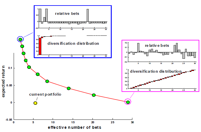
This efficient frontier is similar in spirit to the well-known Markowitz mean-variance efficient frontier, with volatility replaced by the effective number of bets as a risk measure.
Risk factor parity portfolio
Roncalli and Weisang11 and Lohre et al.14 note that a portfolio can be:
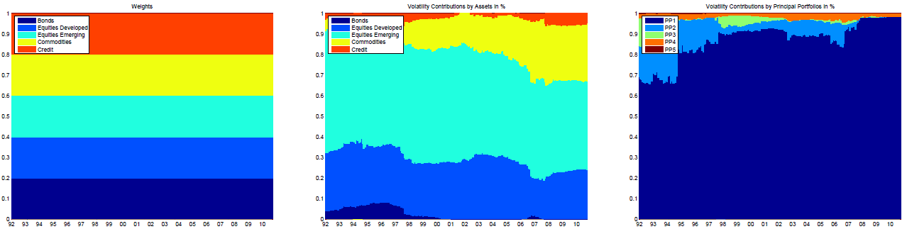
- Perfectly balanced in terms of asset weights, but not at all in terms of risk contributions of its assets, as illustrated in Figure 1 taken from Lohre et al.14 for an equal-weighted multi-asset class portfolio
- Perfectly balanced in terms of risk contributions of its assets, but not at all in terms of risk contributions of its implicit risk factors, as illustrated in Figure 2 also taken from Lohre et al.14 for an equal risk contributions multi-asset class portfolio
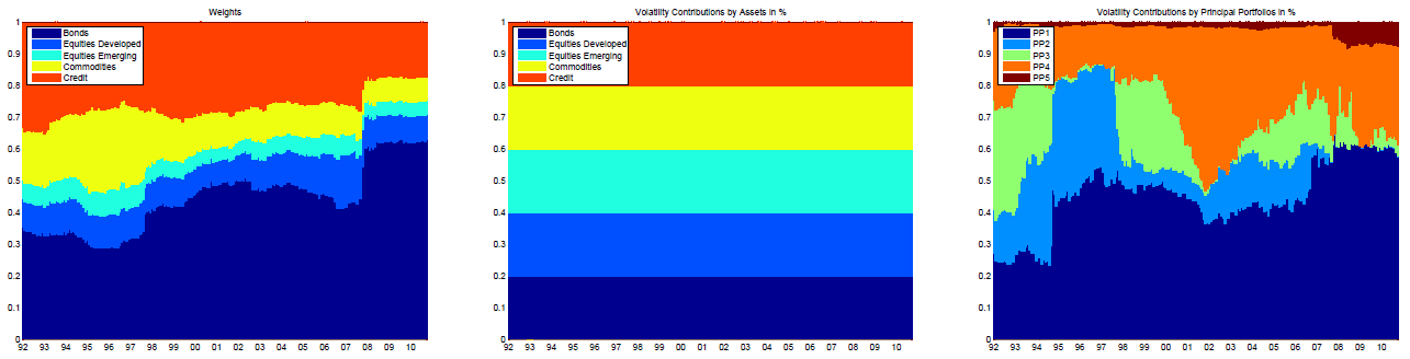
They further note that this situation is typical of risk-based portfolios (equal weighted portfolio, equal risk contributions portfolio, most diversified portfolio…).
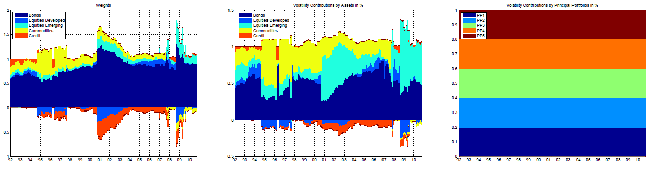
Building on the work of Attilio Meucci, they introduce a new type of risk-based portfolio15 that they call the risk factor parity portfolio11, or the diversified risk parity portfolio14, which aims to be perfectly balanced in terms of risk contributions of its implicit risk factors.
This portfolio corresponds to the maximally diversified portfolio on the mean-diversification efficient frontier proposed by Meucci3.
Figure 4, again taken from Lohre et al.14, illustrates that the risk contributions of the implicit risk factors are indeed all equal for a risk factor parity multi-asset class portfolio.
Conclusion
Anecdotally, I find that the ENB - in its minimum torsion flavor - tends to overestimate the degree of diversification of a portfolio, so that I would recommend to always complement it with an analysis of the dimensionality of the considered universe of assets.
As an illustration, let’s consider an equal-weighted portfolio invested in the following universe of bond ETFs:
- iShares 1-3 Year Treasury Bond ETF - SHY
- iShares 7-10 Year Treasury Bond ETF - IEF
- iShares 20+ Year Treasury Bond ETF - TLT
- iShares TIPS Bond ETF - TIP
- iShares iBoxx $ Investment Grade Corporate Bond ETF - LQD
- iShares iBoxx $ High Yield Corporate Bond ETF - HYG
- iShares National Muni Bond ETF - MUB
From the look of it, this portfolio seems diversified among different type of issuers (government-issued, federal-issued, corporate-issued), different type of maturities, etc., and the ENB seems to confirm this first impression, with an effective number of minimum torsion bets equal to ~6.56 over a theoretical maximum of 716.
Unfortunately, as Horizon Kinetics put it in their 2nd Quarter 2022 Commentary
Maximum diversification means […] maximum exposure to systemic risks. For example, no matter how many individual bonds you own, whatever the mix of corporates, tax-exempts and governments, all their prices will fall when interest rates rise.
While the proper analytical framework to highlight this interest-rate dependency is certainly the analysis of the portfolio exposures to economic factors (inflation, interest rates…), the ENB still gives a false sense of diversification17.
Now, it happens that the effective dimensionality of the considered universe is ~2.22, as measured by the effective rank of the asset covariance matrix16.
So, what the ENB is really indicating is that the portfolio is diversified in terms of implicit risk factors, but only within a universe of ~2 true bond ETFs, very far from the original universe of 7 bond ETFs!
In other words, a high value of the ENB in case of massive hidden redundancy in the considered universe of assets needs to be taken with a grain of salt.
Notes:
- Still anecdotally, I find that the ENB - in its principal components flavor - does not suffer from the same bias. That is, when the effective number of principal components bets indicates that a portfolio is diversified, it usually is. This is consistent with the usage of the (transpose of the) matrix of principal components as the decorrelation matrix in both Roncalli and Weisang11 and Lohre et al.14.
–
-
See Woerheide W, Persson D (1993), An Index of Portfolio Diversification, Financial Services Review 2(2), 73-85. ↩
-
See Yves Choueifaty and Yves Coignard, Toward Maximum Diversification, The Journal of Portfolio Management Fall 2008, 35 (1) 40-51. ↩
-
See Meucci, Attilio, Managing Diversification (April 1, 2010). Risk, pp. 74-79, May 2009, Bloomberg Education & Quantitative Research and Education Paper. ↩ ↩2 ↩3 ↩4 ↩5
-
With the convention that $0 \ln(0) = 0$. ↩
-
This situation is comparable to the situation arising when measuring portfolio risk factor exposures through linear regression analysis, see this blog post. ↩
-
See Meucci, Attilio and Santangelo, Alberto and Deguest, Romain, Risk Budgeting and Diversification Based on Optimized Uncorrelated Factors (November 10, 2015). ↩ ↩2 ↩3 ↩4 ↩5 ↩6 ↩7 ↩8 ↩9 ↩10 ↩11
-
The term synthetic assets is borrowed from Roncalli and Weisang11. ↩
-
This matrix is also called a decorrelating torsion matrix in Meucci et al.6. ↩
-
For example, Meucci et al.6 mention the inverse of the lower triangular Cholesky factor of the asset covariance matrix $\Sigma$. ↩
-
Meucci3 and Meucci et al.6 refer to the principal component decomposition of the asset covariance matrix $\Sigma$, but the matrix $e$ is also the change of basis matrix associated to the diagonalization of $\Sigma$. ↩
-
See Roncalli, Thierry and Weisang, Guillaume, Risk Parity Portfolios with Risk Factors (September 21, 2012). ↩ ↩2 ↩3 ↩4 ↩5
-
This will be the subject of another post. ↩
-
In terms of normalized tracking error, c.f. Meucci et al.6. ↩
-
See Lohre, Harald and Opfer, Heiko and Orszag, Gabor, Diversifying Risk Parity (November 7, 2013). Journal of Risk, Vol. 16, No. 5, 2014, pp. 53-79. ↩ ↩2 ↩3 ↩4 ↩5 ↩6
-
To be noted that expected returns are not taken into account in the computation of the risk factor parity portfolio, so that it belongs to the family of risk-based portfolios. ↩
-
Prices data used for this computation have been retrieved from Tiingo, and are for the period 2021-07-28 to 2022-07-28. ↩ ↩2
-
Although the effective number of principal components bets of the portfolio is ~1.22, which shows a lack of diversification that could be interpreted as a strong exposure of the portfolio to its first principal component, this result is not reliable as discussed in the previous sections. ↩