Mean-Variance Optimization in Practice: Well Diversified (Near) Efficient Portfolios

One well-known stylized fact of the Markowitz’s mean-variance framework is that, irrespective of the quality of the estimates of asset returns and (co)variances, efficient portfolios are concentrated in a very few assets¹.

From a practitioner’s perspective, this has always been a problem¹².

In this blog post, I will describe a solution proposed in Corvalan³, which is to replace efficient portfolios by near efficient portfolios equivalent in terms of risk-return but less concentrated in terms of asset weights.

Notes:

• A Google sheet corresponding to this post is available here

Near optimal mean-variance portfolios

Definition

The output of a mean-variance portfolio optimization procedure is usually a unique⁴ optimal portfolio.

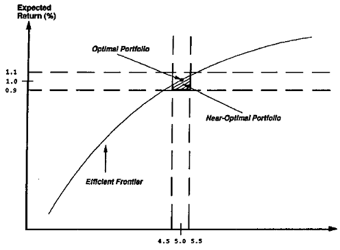
The neighborhood of such a portfolio in the (V,E) plane is called the region of near optimal portfolios⁵ associated to the original optimal portfolio, as illustrated in Figure 1 taken from Chopra⁵.

Figure 1. Region of near optimal portfolios within a 10% window of risk-return around an optimal portfolio. Source: Chopra

Notes:

• While Figure 1 is representative of the general idea of neighborhood, the exact definition depends on the application.

Empirical properties

Several empirical properties of near optimal portfolios have been established in the literature:

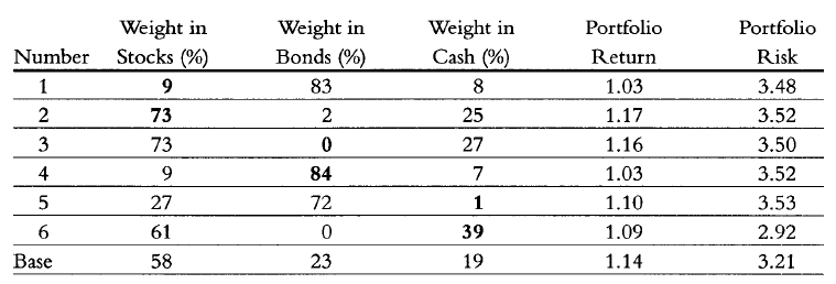
• Near optimal portfolios share similar risk-return characteristics but differ in asset composition. This is illustrated in Chopra⁵, from which Figure 2 is reproduced.

Figure 2. Example of near optimal portfolios belonging to a 10% window of risk-return centered around an optimal portfolio. Source: Chopra

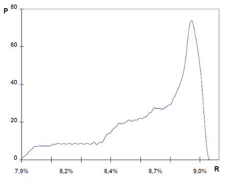
• The region of near optimal portfolios is the most dense region in the (V,E) plane in terms of the number of existing portfolios. This is formally demonstrated in Corvalan³, from which Figure 3 is reproduced.

Figure 3. Holding the level of risk fixed and varying the level of return, the region in the (V,E) plane with the highest number of portfolios (~75) is the region close to the optimal portfolio whose return is equal to 8.97%. Source: Corvalan

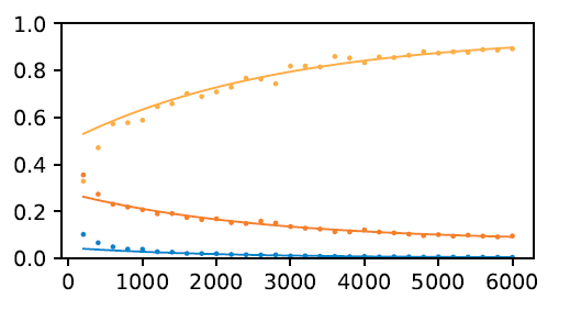
• Near optimal portfolios are significanlty more robust to errors in the estimates of asset returns and (co)variances than the original optimal portfolio. This is analyzed by Van Der Schans and De Graaf⁶, from which figure 4 is reproduced.

Figure 4. The top yellow curve shows that between 60% and 90% of near optimal portfolios remain near optimal after a slight perturbation of asset returns and (co)variances used in the mean-variance optimization procedure. Source: Van Der Schans and De Graaf

Computing diversified near optimal mean-variance portfolios

Building upon the empirical properties of near optimal portfolios, Corvalan³ proposes a two step optimization procedure to compute what he calls well diversified efficient portfolios⁷.

Step 1: Mean-variance optimization

Let be:

• $n$, the number of assets
• $\mu \in \mathbb{R}^{n}$, the vector of the assets arithmetic returns
• $\Sigma \in \mathcal{M}(\mathbb{R}^{n \times n})$, the asset covariance matrix

The first step consists in computing the asset weights $w^* \in \mathbb{R}^{n}$ of an optimal mean-variance portfolio, with return $\mu^{*} = w^* {}^t \mu$ and variance ${\sigma^{*}}^2 = w^* {}^t \Sigma w^* $.

Step 2: Diversification optimization

Let now be:

• $\delta_{\mu} \in \mathbb{R}^{+}$ a relative tolerance over the mean-variance optimal portfolio return $\mu^*$
• $\delta_{\sigma} \in \mathbb{R}^{+}$ a relative tolerance over the mean-variance optimal portfolio standard deviation $\sigma^*$

The second step consists in computing the most diversified⁸ portfolio belonging to the region of near optimal portfolios illustrated in Figure 5.

Figure 5. Region of near optimal portfolios considered in the diversification optimization step.

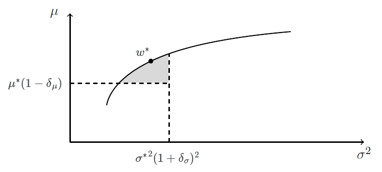
More formally, and for example if the diversification measure is the Herfindahl-Hirschman Index, the asset weights $w^{**} \in \mathbb{R}^{n}$ of the most diversified portfolio are the solution of the following optimization program:

\[w^{**} = \operatorname{argmin} \sum_{i=1}^{n} w_i^2 \newline \textrm{s.t. } \begin{cases} w {}^t \Sigma w \leqslant {\sigma^*}^2 (1 + \delta_{\sigma})^2 \newline \mu^* (1 - \delta_{\mu}) \leqslant w {}^t \mu \newline ... \end{cases}\]

Notes:

• The size of the region of near optimal portfolios is controlled by the parameters $\delta_{\mu}$ and $\delta_{\sigma}$. Intuitively, the higher the uncertainty on the estimates of the asset returns and (co)variances, the greater these parameters should be.
• The Herfindahl-Hirschman Index has been chosen as the portfolio diversification measure in Portfolio Optimizer because it is related to the information content of the portfolio in the sense of information theory, as described in Bouchaud and al.⁹.

Conclusion - Optimal portfolio v.s. diversified near optimal portfolio

Now the one million dollar question.

Should optimal portfolios be replaced altogether by diversified near optimal portfolios?

While anyone will certainly have his own opinion, I would tend to agree.

I will illustrate my reasoning thanks to a simulation made with Portfolio Optimizer and using the weekly closing prices¹⁰ of the four ETFs SPY, TLT, GLD and SHY over the period 2015 - 2021.

At the end of every 12 weeks (~1 quarter):

• I compute the average weekly return of the ETFs over the next 12 weeks, using the Portfolio Optimizer endpoint /assets/returns/average
• I compute the covariance matrix of the ETFs over the next 12 weeks, using the Portfolio Optimizer endpoint /assets/covariance/matrix
• I compute both the maximum Sharpe ratio portfolio and the diversified near maximum Sharpe ratio portfolio associated to these inputs, using the Portfolio Optimizer endpoints /portfolio/optimization/maximum-sharpe-ratio and /portfolio/optimization/maximum-sharpe-ratio/diversified
• I let the resulting portfolios drift for the next 12 weeks

The cumulative profit associated to these two strategies is depicted in Figure 6.

Figure 6. Maximum Sharpe ratio portfolio v.s. diversified near maximum Sharpe ratio portfolio.

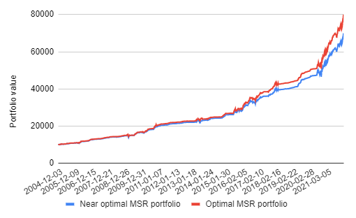
It is quite apparent that little harm is done over the studied ~15 years period by systematically replacing the maximum Sharpe ratio portfolio with its diversified counterpart…

So, if this experiment is representative of a “worst case harm”, and I think it is, then, because of the uncertainty in the estimation of future asset returns and (co)variances, there must be value in replacing optimal portfolios by diversified near optimal portfolios.

As Bouchaud and al. put it⁹:

The problem [with mean-variance optimization] is that one usually has only partial information: past data have a finite length, therefore the determination of statistical parameters is imperfect; predictions of future volatilities and returns are obviously not entirely trustworthy – this is why the optimal portfolio must reflect this lack of information and keep a minimal degree of diversification.

Happy diversification !

–

1. See F. Black and R. Litterman, Global Portfolio Optimization, Financial Analysts Journal, Vol. 48, No. 5 (Sep. - Oct., 1992), pp. 28-43. ↩ ↩²

2. See Michaud, Richard O., The Markowitz Optimization Enigma: Is ‘Optimized’ Optimal? (1989). Financial Analysts Journal, 1989. ↩

3. See A. Corvalan, 2005, Well Diversified Efficient Portfolios,Working Papers Central Bank of Chile 336, Central Bank of Chile. ↩ ↩² ↩³

4. Unless the covariance matrix of the assets is not positive semi-definite. ↩

5. See V. K. Chopra, Improving Optimization, The Journal of Investing Fall 1993, 2 (3) 51-59. ↩ ↩² ↩³

6. See Van Der Schans, M., De Graaf, T., Robust Optimization by Constructing Near-Optimal Portfolios. ↩

7. Which actually needs to be understood as well diversified near efficient portfolios! ↩

8. Most diversified in terms of asset weights. ↩

9. See Bouchaud, J.-P., Potters, M., Aguilar, J.-P., Missing Information and Asset Allocation, arXiv, 1997. ↩ ↩²

10. Adjusted for splits and dividends. ↩