The Turbulence Index: Regime-based Partitioning of Asset Returns

12 minute read

The turbulence index, introduced in the previous blog post, is a measure of statistical unusualness of asset returns popularized by Kritzman and Li¹. It provides a way to measure how much the behavior of a group of assets differs from its historical pattern.

In this post, based on the paper Optimal Portfolios in Good Times and Bad by Chow et al.², I will describe how the turbulence index can be used to partition a set of asset returns into different subsets, each of them corresponding to a specific market risk regime.

I will also provide two examples of usage, one in portfolio optimization and one in the modeling of asset returns.

Mathematical preliminaries

Definitions

Let be:

$n$, the number of assets in a given universe of assets
$T$, the number of time periods
$y_t \in \mathbb{R}^{n}$, the asset returns observed over the time period $t$, $t=1..T$
$\mu \in \mathbb{R}^{n}$, the mean vector of the asset returns over the $T$ periods
$\Sigma \in \mathcal{M}(\mathbb{R}^{n \times n})$, the covariance matrix of the asset returns over the $T$ periods

The (raw) turbulence index $d(y_t)$ for the universe of assets and for a given period $t=1..T$ is defined as the squared Mahalanobis distance²:

\[d(y_t) = (y_t - \mu) {}^t \Sigma^{-1} (y_t - \mu)\]

Mathematical properties

The main mathematical property of the turbulence index relevant for this post³ is the following²:

Property 1: If the asset returns $y_t$ follow a multivariate Gaussian distribution, that is, $y_t \sim \mathcal{N} \left( \mu, \Sigma \right)$, the turbulence index $d(y_t)$ follows a chi-square distribution with $n$ degrees of freedom, that is, $d(y_t) \sim \mathcal{X}^2(n)$.

A method to partition asset returns by regimes based on the turbulence index

Description

Chow et al.² describe how to use the turbulence index to identify multivariate outliers from a series of asset returns. These outliers, that are characterized by the unusual performance of an individual asset or from the unusual interaction of a combination of assets, none of which are necessarily unusual in isolation² are representative of a [turbulent⁴ market] risk regime while the inliers are representative of a quiet market risk regime².

In more details, the method of Chow et al.² partitions a set of multivariate asset returns $y_t \in \mathbb{R}^{n}, t=1..T$ into two subsets corresponding to these two regimes as follows:

Compute the mean vector $\mu$ of the asset returns
Compute the covariance matrix $\Sigma$ of the asset returns
Choose a turbulence threshold $tt$%, which represents the percentage of asset returns desired to be classified as quiet, with typical value 70%, 80%, 95%⁵…
Convert the turbulence threshold $tt$% into a turbulence score $ts$
For each asset return vector $y_t, t=1..T$:
- Compute the turbulence index value $d(y_t)$
- If $d(y_t) \leq ts$, $y_t$ is classified as belonging to the quiet regime; otherwise, if $d(y_t) > ts$, $y_t$ is classified as belonging to the turbulent regime

How to convert the turbulence threshold into a turbulence score?

The turbulence threshold $tt$% is not directly comparable to the turbulence index values $d(y_t)$, $t=1..T$ because they are not expressed in the same units⁶.

As a consequence, $tt$% needs to be converted into a turbulence score $ts$.

Under the assumption that the asset returns $y_t$ follow a multivariate Gaussian distribution, and based on Property 1, this conversion can be done by thanks to the computation of the $tt$-th percentile of the chi-square distribution with $n$ degrees of freedom, that is,

\[ts = \left( \mathcal{X}^2(n) \right)^{-1} (tt)\]

Nevertheless, because asset returns do not follow a multivariate Gaussian distribution in practice⁷, this conversion will result in a proportion of asset returns classified as quiet that is different from the desired proportion.

This problem is highlighted in Chow et al.², in which a turbulence threshold of 75% is used to separate outliers from inliers while the actual proportion of asset returns classified as quiet v.s. turbulent is equal to 79.1%.

A possible solution is to convert the turbulence threshold $tt$% into a turbulence score thanks to the computation of the $tt$-th empirical percentile of the turbulence index distribution⁸⁹, with the caveat that this solution requires a long enough series of asset returns.

Illustration

I will illustrate the method of Chow et al.² with a simple two-asset universe made of:

U.S. stocks (SPY ETF)
U.S. 20+ year Treasuries (TLT ETF)

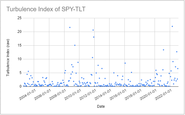
The turbulence index for this universe of assets, computed using monthly returns over the period August 2002 - January 2023¹⁰, is represented in Figure 1.

Figure 1. SPY-TLT turbulence index, August 2002 - January 2023.

Then, using for example a turbulence threshold $tt$% of 80%, converted into a turbulence score $ts$ of ~3.22¹¹:

All pairs of SPY-TLT returns whose turbulence index is below the red line depicted in Figure 2 are classified as belonging to the quiet regime
All pairs of SPY-TLT returns whose turbulence index is strictly above the red line depicted in Figure 2 are classified as belonging to the turbulent regime

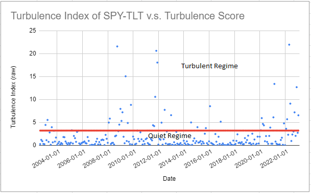
Figure 2. SPY-TLT turbulence index v.s. turbulence score of 80%, August 2002 - January 2023.

This partitioning of the SPY-TLT returns seems to make some sense, as several periods of market stress are identifiable within the turbulent regime: the Global Financial Crisis, the COVID-19 pandemic, the Russian invasion of Ukraine…

Implementation in Portfolio Optimizer

Portfolio Optimizer implements the method from Chow et al.² through the endpoint /assets/returns/turbulence-partitioned, with two extensions:

Several turbulence thresholds $tt_i$%, $i=1..m$, $m \geq 1$ can be provided, in which case the initial set of asset returns is partitioned into (at most) $m+1$ subsets¹²
Turbulence threshold(s) can be converted into turbulence score(s) thanks to the computation of the empirical percentiles of the turbulence index distribution, as described in Kritzman et al.⁸⁹

Examples of application

Being able to partition asset returns into different market risk regimes has several applications.

For example, it allows to analyze the potential behavior of a given portfolio during periods of market stress, which is of utmost importance for long-term investing.

As Chow et al.² puts it:

[a] portfolio may not survive to generate long-term performance if [it] cannot withstand exceptional periods of market turbulence.

I will not insist on this specific example, though, but I will provide one example related to portfolio optimization and one example related to the modeling of asset returns.

Building mean-variance optimal and regime-sensitive portfolios

Under the Markowitz’s mean-variance framework, building an optimal portfolio within a universe of assets requires an estimation of the asset covariance matrix.

Because [the] typical risk-estimation procedure […] is to weight a sample [of asset returns]’ observations equally in order to estimate risk parameters², the expected volatility of such a portfolio during periods of market stress, when asset returns typically become more volatile and more correlated, will be underestimated.

This situation is illustrated in Figure 3, taken from Chow et al.², in the case of a universe of assets made of eight distinct asset classes¹³.

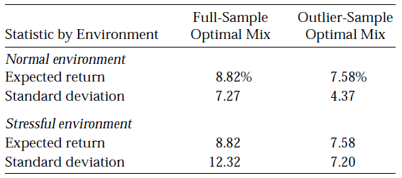
Figure 3. Impact of full sample v.s. turbulent sample asset covariance matrix estimation on a mean-variance optimal portfolio. Source: Chow et al.

In this figure, it can be seen that an optimal portfolio whose asset covariance matrix is estimated from a non-partitioned set of asset returns (Full-Sample Optimal Mix) sees its volatility skyrocket during periods of market stress (Stressful environment) when compared to periods of market stability (Normal environment).

One solution to this issue is to estimate the asset covariance matrix from only the subset of asset returns corresponding to periods of market stress, but in this case, the expected portfolio return might be negatively impacted.

Indeed, as can also be seen in Figure 3, an optimal portfolio whose asset covariance matrix is estimated from only the subset of asset returns corresponding to periods of market stress (Outlier-Sample Optimal Mix) sees its expected return diminished by $\approx 1.24$% compared to the previous optimal portfolio (Full-Sample Optimal Mix).

Another solution, suggested by Chow et al² and Kritzman et al.⁹, is to estimate a blended asset covariance matrix from both¹⁴:

The subset of asset returns corresponding to periods of market stress
The subset of asset returns corresponding to periods of market stability

More specifically, these papers suggest to estimate an asset covariance matrix $\Sigma^*$ equal to

\[\Sigma^* = \lambda_{i}^* p_{i} \Sigma_{i} + \lambda_{o}^* \left( 1 - p_{i} \right) \Sigma_{o}\]

, where:

$\lambda_i^*$ (resp. $\lambda_o^*$) is the relative¹⁵ risk aversion of investors to the quiet (resp. turbulent) regime
$p_{i}$ (resp. $1 - p_{i}$¹⁶) is the probability that the next period’s regime is quiet (resp. turbulent)
$\Sigma_{i}$ is the quiet regime asset covariance matrix, estimated from the subset of asset returns corresponding to the quiet regime
$\Sigma_{o}$ is the turbulent regime asset covariance matrix, estimated from the subset of asset returns corresponding to the turbulent regime

Such a blended covariance matrix enables investors to express their views about the likelihood of each risk regime and to differentiate their aversion to the regimes².

Now, in practice, the computation of $\Sigma^*$ requires to estimate the probability $p_{i}$.

This can be done in an ad-hoc fashion, or using one’s preferred forecast technique, like the hidden Markov model used in Kritzman et al.⁹.

A couple of remarks to finish:

Under the Markowitz’s mean-variance framework, building an optimal portfolio within a universe of assets also requires an estimation of the expected asset returns.

They are assumed to be regime-independent in Chow et al.², but they could perfectly be made conditional on the regime like in Bruder et al.¹⁷.
In the specific case where investors are equally averse to both the quiet and the turbulent regime, the formula for $\Sigma^*$ simplifies to

\[\Sigma^* = p_{i} \Sigma_{i} + \left( 1 - p_{i} \right) \Sigma_{o}\]

Fitting the parameters of a multivariate Gaussian mixture distribution

It has been known since the early 1960s that the (marginal) statistical distribution of asset returns is neither normal nor lognormal⁷, but more than sixty years later it is still an open question in financial mathematics to determine its exact nature.

Empirically, though, it has been demonstrated that several distributions are able to capture most of the stylized facts¹⁸ of asset returns.

One such distribution is the Gaussian mixture distribution, which is a convex combination of Gaussian distributions with different means and variances in the univariate case and a a convex combination of multivariate Gaussian distributions with different mean vectors and covariance matrices in the multivariate case.

The main advantages of this distribution over other alternatives like the multivariate t distribution is that it is a non-elliptical distribution¹⁹ both numerically tractable²⁰ and extremely flexible.

For example, a univariate Gaussian mixture distribution can be unimodal, symmetric, skewed, multimodal, leptokurtic…²¹.

As another example, a multivariate Gaussian mixture distribution with two components allows to approximate a multivariate jump-diffusion model driven by a standard Lévy process¹⁷.

In this context, the method of Chow et al.² can be applied to fit the parameters of a two-component²² multivariate Gaussian mixture distribution as detailed below²³:

Set the weights of the two components respectively to the turbulence threshold $tt$%²⁴ and its complement $1 - tt$%
Estimate the mean vector and the covariance matrix of the multivariate Gaussian distribution with component weight $tt$% by their sample counterparts computed on the quiet subset of asset returns
Estimate the mean vector and the covariance matrix of the multivariate Gaussian distribution with component weight $1 - tt$% by their sample counterparts computed on the turbulent subset of asset returns

In order to illustrate the validity of this approach on the two-asset SPY-TLT universe introduced in the previous section, Figure 4 through Figure 6 compare the empirical distribution of the monthly SPY (log) returns with the first marginal of:

A multivariate Gaussian distribution fitted to the pairs of SPY-TLT returns with maximum likelihood estimation

Figure 4. Monthly SPY log returns, empirical c.d.f. v.s. Gaussian c.d.f. fitted with maximum likelihood estimation, August 2002 - January 2023.

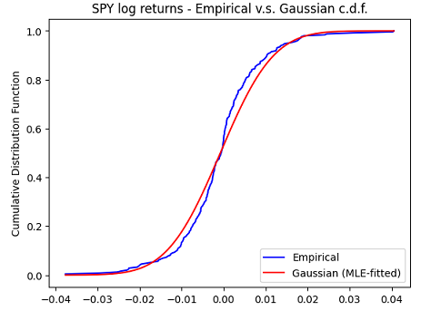
A multivariate Gaussian mixture distribution fitted to the pairs of SPY-TLT returns with the turbulence index-based methodology above using a turbulence threshold of 80%²⁵

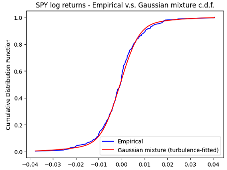
Figure 5. Monthly SPY log returns, empirical c.d.f. v.s. Gaussian mixture c.d.f. fitted with the turbulence index-based methodology, August 2002 - January 2023.

A multivariate Gaussian mixture distribution fitted to the pairs of SPY-TLT returns with the expectation–maximization algorithm²⁶

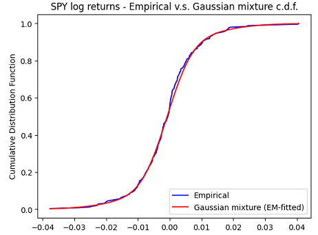
Figure 6. Monthly SPY log returns, empirical c.d.f. v.s. Gaussian mixture c.d.f. fitted with the expectation–maximization algorithm, August 2002 - January 2023.

It is clearly visible on these figures that both marginal Gaussian mixture distributions are much more appropriate than the marginal Gaussian distribution to model the SPY returns, with a slightly better fit obtained with the expectation–maximization algorithm.

This is confirmed numerically by the Kolmogorov-Smirnov goodness of fit test²⁷.

Going beyond univariate marginals, a 2D Kolmogorov-Smirnov goodness of fit test²⁸ also confirms that both multivariate Gaussian mixture distributions are much more appropriate than the multivariate Gaussian distribution to model the joint SPY-TLT returns²⁹, with a slightly better fit again obtained with the expectation–maximization algorithm.

This example shows that it is possible to fit the parameters of a multivariate Gaussian mixture distribution modeling joint asset returns through an easily interpretable procedure, with no local optima and no convergence issue to worry about³⁰.

Conclusion

This concludes this second post on the turbulence index.

As usual, feel free to connect with me on LinkedIn or follow me on Twitter to discuss about Portfolio Optimizer or quantitative finance in general.

–

See M. Kritzman, Y. Li, Skulls, Financial Turbulence, and Risk Management,Financial Analysts Journal, Volume 66, Number 5, Pages 30-41, Year 2010. ↩
See George Chow, Jacquier, E., Kritzman, M., & Kenneth Lowry. (1999). Optimal Portfolios in Good Times and Bad. Financial Analysts Journal, 55(3), 65–73.. ↩ ↩² ↩³ ↩⁴ ↩⁵ ↩⁶ ↩⁷ ↩⁸ ↩⁹ ↩¹⁰ ↩¹¹ ↩¹² ↩¹³ ↩¹⁴ ↩¹⁵ ↩¹⁶ ↩¹⁷
For other properties, c.f. the first blog post of this series. ↩
The turbulent regime is called stressful in Chow et al.². ↩
To be noted that $1 - tt$% is used in Chow et al.² as the turbulence threshold, and not directly $tt$%. ↩
The turbulence threshold is expressed as a percentage, while the turbulence index is expressed as a squared Mahalanobis distance. ↩
See Mandelbrot B, The variation of certain speculative prices, The Journal of Business, 1963, vol. 36, 394. ↩ ↩²
See M. Kritzman, Y. Li, Skulls, Financial Turbulence, and Risk Management,Financial Analysts Journal, Volume 66, Number 5, Pages 30-41, Year 2010. ↩ ↩²
See Mark Kritzman, Kenneth Lowry and Anne-Sophie Van Royen, Risk, Regimes, and Overconfidence, The Journal of Derivatives Spring 2001, 8 (3) 32-42. ↩ ↩² ↩³ ↩⁴
I retrieved the monthly adjusted ETF prices over the period July 2002 - January 2023 using Tiingo. ↩
Using for example the Matlab function chi2inv, chi2inv(0.80,2) = 3.218875824868201. ↩
For example, Kinlaw et al.³¹ use, although in a slightly different context, three subsets corresponding to the three market risk regimes calm, moderate and turbulent. ↩
The eight asset classes are Domestic equities, Foreign equities, Emerging market, Domestic bonds, Foreign bonds, High-yield bonds, Commodities and Cash. ↩
Or from all the subsets of asset returns corresponding to all the market regimes in case more than two turbulence thresholds are used. ↩
In Chow et al², the relative risk aversion parameters are actually rescaled so that they sum to 2, that is, they must verify $\lambda_{i}^* + \lambda_{p}^* = 2$. ↩
Because Chow et al² consider only two regimes, $p_{o} = 1 - p_{i}$. ↩
See Bruder, Benjamin and Kostyuchyk, Nazar and Roncalli, Thierry, Risk Parity Portfolios with Skewness Risk: An Application to Factor Investing and Alternative Risk Premia (September 22, 2016). ↩ ↩²
See R. Cont (2001) Empirical properties of asset returns: stylized facts and statistical issues, Quantitative Finance, 1:2, 223-236. ↩
See Ian Buckley, David Saunders, Luis Seco, Portfolio optimization when asset returns have the Gaussian mixture distribution, European Journal of Operational Research, Volume 185, Issue 3, 2008, Pages 1434-1461. ↩
Because it is “just” an extension of the Gaussian model, calculations with this distribution are usually similar to those using the Gaussian distribution. ↩
See Gaussian mixtures and financial returns, C. Cuevas-Covarrubias, J. Inigo-Martinez, R. Jimenez-Padilla, Discussiones Mathematicae, Probability and Statistics 37 (2017) 101–122. ↩
Or of a multivariate Gaussian mixture distribution with more than two components in case more than two turbulence thresholds are used. ↩
This approach is similar in spirit to the thresholding method of Bruder et al.¹⁷. ↩
Or, for more robustness in case the chi-square distribution is used to convert the turbulence threshold into a turbulence score, to the actual proportion of asset returns qualified as quiet v.s. turbulent. ↩
This turbulence threshold results in an actual proportion of asset returns that qualify as quiet v.s. turbulent equal to ~0.83%. ↩
Thanks to the Python Scikit-Learn package. ↩
The Kolmogorov-Smirnov statistic (resp. p-values) for the three marginal distributions are, in order ~0.0892, ~0.0544, ~0.0527 (resp. ~0.0373, ~0.4437, ~0.4852). ↩
Using the Python library https://github.com/syrte/ndtest. ↩
The 2-sample 2D Kolmogorov-Smirnov p-values²⁸ are usually ~< 0.01 for the multivariate Gaussian distribution and much greater than ~0.20 for both multivariate Gaussian mixture distributions, indicating that the joint SPY-TLT returns distribution is significantly different from the former and not significantly different from any of the latter. ↩
See Hichem Snoussi, Ali Mohammad-Djafari, Penalized maximum likelihood for multivariate Gaussian mixture, arXiv. ↩
See William Kinlaw, Mark P. Kritzman, David Turkington, Harry M. Markowitz, A Practitioner’s Guide to Asset Allocation, Wiley. ↩