The Absorption Ratio: Measuring Financial Risk, Part 2

7 minute read

In the previous post, I reviewed the turbulence index, an indicator of financial market stress periods based on the Mahalanobis distance, introduced by Chow et al.¹ and Kritzman and Li².

In this post, I will review the absorption ratio, a measure of financial market fragility based on principal components analysis, introduced by Kritzman et al.³. I will also show how to compute this absorption ratio for the U.S. stock market and how it could be used to scale the market exposure of a portfolio of U.S. equities.

Mathematical preliminaries

Definition

Let be:

$n$, the number of assets in a given universe of assets
$\Sigma \in \mathcal{M}(\mathbb{R}^{n \times n})$, the asset covariance matrix
$E_1,…,E_n$, the eigenvectors of $\Sigma$ ordered such that $\sigma_{E_1}^2 \geq … \geq \sigma_{E_n}^2$, with $\sigma_{E_i}^2$ the variance of the eigenvector $E_i$, $i=1..n$
$1\leq N \leq n$, the number of eigenvectors $E_1,…,E_N$ to retain in the computation of the absorption ratio

The absorption ratio $AR$ of the universe of assets is defined³ as the fraction of the total variance of the assets explained (or absorbed, hence its name) by the finite set of eigenvectors $E_1,…,E_N$.

\[AR = \frac{\sum_{i=1}^N \sigma_{E_i}^2}{\sum_{i=1}^n \sigma_{E_i}^2}\]

Notes:

The denominator of the absorption ratio $AR$ is also equal to $\sum_{i=1}^n \sigma_{A_i}^2$, with $\sigma_{A_i}^2$ the variance of the $i$-th asset, $i=1..n$, which is its usual definition.

Interpretation

The absorption ratio of a universe of assets can be interpreted as follows:

When the absorption ratio is high, a large part of the variance of the asset returns is explained by the assets exposure to the same source(s) of risk, for example the stock market as a whole, a given sector, a given industry, etc.
When the absorption ratio is low, a large part of the variance of the asset returns is explained by the assets individual characteristics

So, the absorption ratio measures how concentrated the risk is in a universe of assets, which helps to:

Determine whether a universe of assets is “fragile” or “resilient”.

As Marc Kritzman puts it⁴:

When assets are tightly coupled, they are collectively fragile, in the sense that negative shocks travel more quickly and broadly than when assets are loosely linked. In contrast, a low absorption ratio implies that risk is distributed broadly across disparate sources; hence, the assets are less likely to exhibit a unified response to bad news.

Measure the diversification potential of a universe of assets, in a similar way to the efficient rank.

Indeed, a universe of assets whose prices move fully in sync provides little diversification benefits…

Empirical properties

Kritzman et al.³ establish several empirical properties of the absorption ratio, for example that major U.S. stock market crashes were preceded by spikes in the absorption ratio.

This property is also established in the 2012 U.S. Treasury Department’s Office of Financial Research (OFR) Annual Report⁵, which analyses the behavior of the absorption ratio of a global universe of assets around several financial crisis and concludes that:

Based on our analysis of four events, [the absorption ratio] tends to drift upward ahead of the crisis and then jump abruptly on the event date, persisting at the new higher level afterward.

How to determine the number of eigenvectors to retain?

When computing the absorption ratio, it is standard practice in the litterature to use a number of eigenvectors of about 1/5th the number of assets³⁶.

That being said, the usage of only one eigenvector is also documented in both the academia⁷⁸ and the industry, an example of the latter being the methodology underlying the construction of the HSBC Risk On-Risk Off (RORO) Index⁹¹⁰.

Personally, for the sake of simplicity, I would advise to retain only one eigenvector in the computation of the absorption ratio, unless there is a strong justification to include more eigenvectors.

U.S. stock market absorption ratio

I will now illustrate how to compute the absorption ratio for the Sector SPDR ETFs¹¹, using the Portfolio Optimizer API.

As these ETFs cover stocks across the S&P 500, the associated absorption ratio should be representative of the U.S. stock market as a whole¹².

I will use the following rolling window approach.

At the end of each week:

The sample covariance matrix $\Sigma$ of the ETFs is computed over the last 52 weeks¹³ of weekly return data, using the Portfolio Optimizer endpoint /assets/covariance/matrix
The associated absorption ratio is computed, using the Portfolio Optimizer endpoint /assets/analysis/absorption-ratio with one eigenvector of $\Sigma$ retained

The resulting absorption ratio over the period October 2000 - March 2022 is displayed in Figure 1, on which 5 major stock market crashes are also labeled.

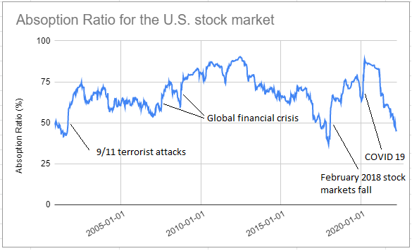
Figure 1. Absorption ratio for the U.S. stock market, October 2000 - March 2022

It appears that:

The absorption ratio tends to decrease just before a stock market crash
The absorption ratio tends to spike during a stock market crash
The absorption ratio tends to stay elevated just after a stock market crash and then to slowly diminish over time

While the two last points above are in agreement with the results from prior research³⁵, the first point is not.

A possible explanation is that the frequency of the return data as well as the size of the window over which the asset covariance matrix is computed both impact the behaviour of the absorption ratio before a stock market crash.

Another possible explanation is that my definition of a decreasing time series does not match with the one used in prior research…

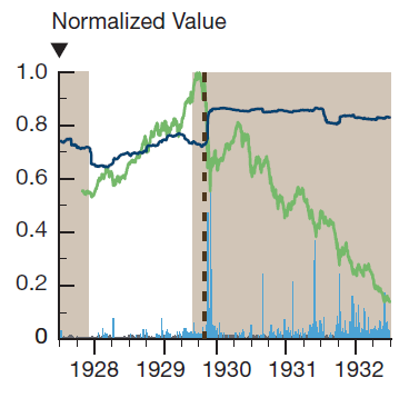
As an example, the 2012 OFR Annual Report⁵ defines the absorption ratio illustrated in figure 2 as being increasing just before the 1929 market crash whereas I define it as being decreasing.

Figure 2. Absorption ratio of global assets around the 1929 crash. Source: 2012 OFR Annual Report

Definitions put aside, and similar to the turbulence index, I find it really interesting that the empirical properties of the absorption ratio seem to be as valid in 2022 as they were in 2011 at the time of their initial publication!

Example of usage - Scaling the market exposure of a portfolio

Kritzman et al.³ note that:

significant increases in the absorption ratio are followed by significant stock market losses, on average, while significant decreases in the absorption ratio are followed by significant gains

Following this observation, they propose a trading strategy consisting in varying the exposure to stocks of a 50% U.S. government bonds/50% U.S. stocks portfolio based on
significant changes in the absorption ratio of the MSCI USA index.

On my side, I propose to integrate the absorption ratio into a more generic trading strategy, capturing the idea that exposure to stocks should be decreased when the absorption ratio is increasing and vice-versa.

The details are as follow.

At the end of each week:

Compute the value of the absorption ratio of the U.S. stock market defined in the previous paragraph
Determine how elevated is this absorption ratio relative to its history¹⁴, on a scale $s$ from 0% to 100%
Allocate $s$% of the portfolio to cash and $1-s$% of the portfolio to U.S. equities

Figure 3 illustrates this strategy with the SPY ETF (U.S. equities) and the SHY ETF (cash) over the period October 2000 - March 2022¹⁵, and compare it to a buy and hold strategy over the same period.

Figure 3. Buy and hold v.s. absorption-ratio-adjusted SPY

Although this strategy struggles when the absorption ratio is choppy, like around 2005 and 2015, it seems to be efficient in managing portfolio risk.

Figures:

Portfolio Management Strategy	Average Exposure	Annualized Sharpe Ratio	Maximum (Weekly) Drawdown
Buy and hold	100%	~0.54	~55%
Absorption-ratio-adjusted	~50%	~0.85	~15%

Conclusion

The absorption ratio is an indicator of financial risk, complementary to the turbulence index.

They both provide warning signals when dangerous periods are ahead on financial markets, signals which can be used to de-risk portfolios.

In a future post, I will analyze the overlap, if any, between these two indicators as well as between these two indicators and the efficient rank.

–

See George Chow, Jacquier, E., Kritzman, M., & Kenneth Lowry. (1999). Optimal Portfolios in Good Times and Bad. Financial Analysts Journal, 55(3), 65–73.. ↩
See M. Kritzman, Y. Li, Skulls, Financial Turbulence, and Risk Management,Financial Analysts Journal, Volume 66, Number 5, Pages 30-41, Year 2010. ↩
See Mark Kritzman, Yuanzhen Li, Sebastien Page and Roberto Rigobon, Principal Components as a Measure of Systemic Risk, The Journal of Portfolio Management Summer 2011, 37 (4) 112-126. ↩ ↩² ↩³ ↩⁴ ↩⁵ ↩⁶
See Mark Kritzman, Risk Disparity, The Journal of Portfolio Management Fall 2013, 40 (1) 40-48. ↩
See Office of Financial Research Annual Report 2012, United States Treasury Department. ↩ ↩² ↩³
See D. Bradfield & D Hendricks (2014) Monitoring Market Fragility Using the Absorption Ratio, Studies in Economics and Econometrics, 38:2, 33-46. ↩
See Zheng, Z., Podobnik, B., Feng, L. et al. Changes in Cross-Correlations as an Indicator for Systemic Risk. Sci Rep 2, 888 (2012). ↩
See Fenn DJ, Porter MA, Williams S, McDonald M, Johnson NF & Jones NS. Temporal evolution of financial-market correlations. Phys. Rev. E 84, 026109, 2011.. ↩
See UOA10-11: Risk On / Risk Off: from academic research to financial market staple. ↩
See Williams S., Fenn D. and McDonald M. (2012) “Risk On-Risk Off: Fixing a Broken Investment Process”, HSBC Global Research, April ↩
I will only use the 9 original sector ETFs, whose associated tickers are XLY, XLP, XLE, XLF, XLV, XLI, XLB, XLK and XLU. ↩
This absorption ratio is similar in spirit to the HSBC Equity RORO Index. ↩
See Zheng et al.⁷ for a discussion about the usage of a short 12-month window in the computation of the absorption ratio. ↩
I will not disclose my implementation details for this step. On their side, Kritzman et al.⁷ compute what they call the standardized shift in the absorption ratio, which is akin to a z-score, and convert it to either 0%, 50% or 100% of exposure to stocks. ↩
The inception date for the SHY ETF is 22th July 2002, so that SHY price data before this date have been taken from the associated index, which is the Barclays U.S. 1-3 Year Treasury Bond Index. ↩