Mean-Variance Optimization in Practice: Reverse Optimization and Implied Expected Returns

The fact that mean-variance optimizers are highly sensitive to changes in expected returns […] is well known in investment practice¹, with a couple of practical solutions already described in this blog, for example using near efficient portfolios or subset resampling-based efficient portfolios.

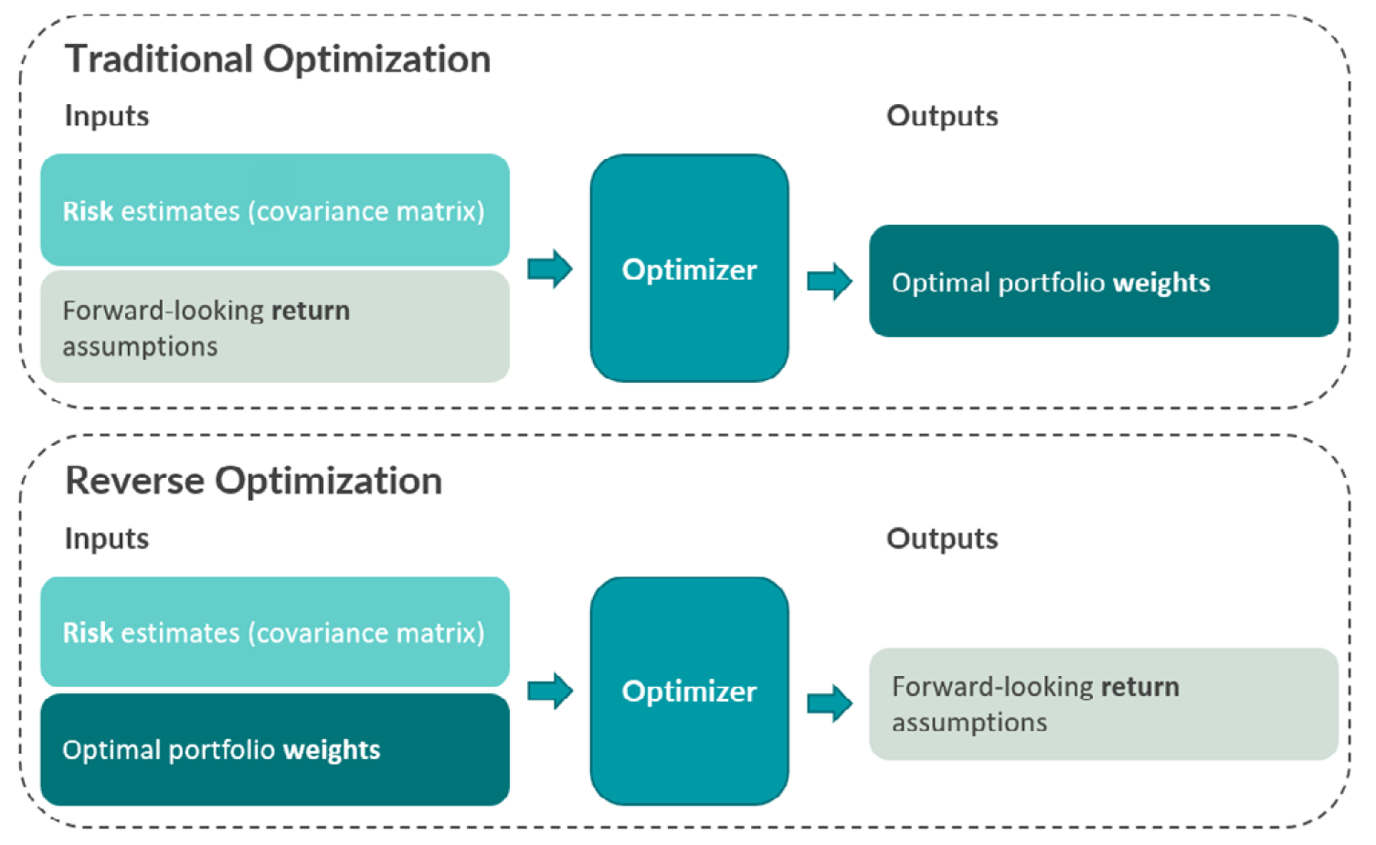
In this blog post, I will introduce another approach originally described in Sharpe² and known as reverse optimization³, which consists in trying to improve the robustness of expected returns estimates by turning the mean-variance optimization problem around.

In more detail, instead of optimizing portfolio weights using a set of expected returns and a covariance matrix⁴, reverse optimization starts with the weights of a given portfolio⁵ and solves for the corresponding set of [implied] expected returns³ that makes it mean–variance efficient.

That approach, illustrated in Figure 1 taken from Two Sigma⁶, has been popularized by the Black-Litterman methodology and has empirically been shown to improve out-of-sample performance of portfolios⁷, c.f. for example Ardia and Boudt⁴ or Ni et al.⁷.

Figure 1. Differences between traditional and reverse mean-variance optimization. Source: Two Sigma.

As a main example of usage, I will show how reverse optimization allows to analyze the hidden assumption made by index investors in the MSCI World w.r.t. future U.S. over ex-U.S. equities performance.

Reverse mean-variance optimization and implied expected returns

Let be:

• $n$, the number of assets in a universe of assets
• $\mu \in \mathbb{R}^{n}$, the vector of expected asset arithmetic returns at a given holding horizon (one day, one month…)
• $\Sigma \in \mathcal{M}(\mathbb{R}^{n \times n})$, the covariance matrix of the asset arithmetic returns at the holding horizon
• $\lambda$, $0 < \lambda < +\infty$, a risk tolerance⁸ parameter

Under the Markowitz’s mean-variance framework, a mean–variance efficient portfolio is defined as a vector of portfolio weights $w^* \in \mathbb{R}^{n}$ that maximizes the mean–variance utility function

\[w^* = \operatorname{argmax} \mu {}^t w - \frac{\lambda}{2} w {}^t \Sigma w \newline \textrm{s.t. } w \in C\]

, where $C \subset \mathbb{R}^{n}$ is the set of investment constraints on the portfolio weights (budget constraint, no short-sale constraint, sector exposure constraints…).

Reverse unconstrained mean-variance optimization

When no constraints are imposed on the mean-variance optimization problem or when no linear constraint is binding at optimality¹², the first-order optimality condition associated to the mean–variance utility function maximisation problem above is

\[\frac{\partial \mathcal{L}}{\partial w} = \mu - \lambda \Sigma w = 0\]

, where $\mathcal{L}(w) = \mu {}^t w - \frac{\lambda}{2} w {}^t \Sigma w$ is the Lagrangian of the mean–variance utility function maximisation problem.

Now, assuming that the solution to this problem $w^* \in \mathbb{R}^{n}$ is known but $\mu$ is not, it is then possible to isolate $\mu$, which leads to the classical¹ definition of the vector of implied expected returns $\mu_{impl} \in \mathbb{R}^{n}$ as

\[\mu_{impl} = \lambda \Sigma w^*\]

Ardia and Boudt⁴ comments that definition as follows:

We thus see that the implied expected return for [a] stock is proportional to the covariance between the stock’s return and the return on the mean–variance efficient portfolio.

Ceteris paribus, this covariance will tend to be higher for stocks that have: (i) a relatively larger weight in the efficient portfolio proxy, (ii) a high volatility, and (iii) a high correlation with the stocks in the efficient portfolio.

The propagation of the weights bets to implied returns bets thus interacts with the variance and correlation properties of the individual stock returns.

Reverse budget-constrained mean-variance optimization

Herold¹ notes that in the literature, implied returns are regularly computed according to [the relationship established in the previous sub-section, which] will often result in unreasonable values¹.

Indeed, the assumption that no constraints are imposed on the mean-variance optimization problem or that no constraints are binding at optimality is not realistic, because in practice the budget constraint is relevant to the investor¹.

So, let be $C = \{ w \in \mathbb{R}^{n}, \sum_{i=1}^n w_i = 1 \}$ representing the budget constraint.

The Lagrangian of the mean–variance utility function maximisation problem then becomes¹⁹

\[\mathcal{L}(w) = \mu {}^t w - \frac{\lambda}{2} w {}^t \Sigma w - \gamma \left( w {}^t 1_n - 1 \right)\]

, where:

• $\gamma \in \mathbb{R}$ is the Lagrange multiplier associated to the budget constraint $\sum_{i=1}^n w_i = 1$
• $1_n$ is a $n$-dimentional vector of 1s

and the first-order optimality condition becomes¹⁹

\[\frac{\partial \mathcal{L}}{\partial w} = \mu - \lambda \Sigma w - \gamma 1_n = 0\]

Consequently, and again assuming that the solution to this problem $w^*$ is known but $\mu$ is not, the vector of implied expected returns $\mu_{impl}$ turns into a two-parameter family that depends on a […] multiplicative factor and an additive component¹:

\[\mu_{impl} = \lambda \Sigma w^* + \gamma 1_n\]

Herold¹ argues¹⁰ that this definition - although involving an additional parameter $\gamma$ - results in sensible and more realistic values for the implied returns¹ than the common procedure of determining the multiplier only and implicitly setting the additive constant to zero¹.

As a side note, under the additional assumption that the marginal investor’s objective is to maximize risk-adjusted returns (or Sharpe Ratio)⁶, it can be shown¹¹ that $\gamma$ can be set to 0, which justifies the widespread use of the definition of $\mu_{impl}$ established in the previous sub-section.

Reverse linearly-constrained mean-variance optimization

Beyond the budget constraint analyzed in the previous sub-section, the standard mean-variance portfolio optimization problem originally introduced in Markowitz¹² involves general linear constraints on the portfolio weights $w$ modelled through the set $C = \{ w \in \mathbb{R}^{n}, Ax = b, Cx \leq d \}$, where:

• $A \in \mathcal{M}(\mathbb{R}^{n_e \times n})$ and $b \in \mathbb{R}^{n_e}$ represent linear equality constraints, like the budget constraint $\sum_{i=1}^n w_i = 1$
• $C \in \mathcal{M}(\mathbb{R}^{n_i \times n})$ and $d \in \mathbb{R}^{n_i}$ represent linear inequality constraints like nonnegativity constraints¹³ $w_i \geq 0, i=1..n$ or sector constraints

While that formulation is apparently much more complex than that of the previous sub-section, Sharpe² actually notes that the solution, once determined, can he characterized as the solution to a [linear equality-constrained] problem², so that only the case $C = \{ w \in \mathbb{R}^{n}, Ax = b \}$ needs to be analyzed.

As Sharpe² puts it:

Inequality constraints not binding in the solution are simply omitted from the expression of the problem; those that were binding are included as equalities.

Thus, assuming that the solution to this problem $w^*$ is known¹⁴, the Lagrangian of the mean–variance utility function maximisation problem becomes²

\[\mathcal{L}(w) = \mu {}^t w - \frac{\lambda}{2} w {}^t \Sigma w - \langle {\Gamma, A' w - b'} \rangle\]

, where:

• $n_b \geq 0$ represents the number of binding inequality and bound constraints at optimality turned into linear equality constraints
• $A’ \in \mathcal{M}(\mathbb{R}^{(n_e + n_b) \times n})$ and $b \in \mathbb{R}^{n_e + n_b}$ represent the original linear equality constraints $(A,b)$ plus the binding inequality and bound constraints at optimality turned into linear equality constraints
• $\Gamma \in \mathbb{R}^{n_e + n_b}$ are the Lagrange multipliers associated to the $n_e + n_b$ equality constraints

and the first-order optimality condition becomes²

\[\frac{\partial \mathcal{L}}{\partial w} = \mu - \lambda \Sigma w - A' {}^t \Gamma = 0\]

This time, the vector of implied expected returns $\mu_{impl}$ turns into a $n_e + n_b + 1$-parameter family that depends on a multiplicative factor and several additive components:

\[\mu_{impl} = \lambda \Sigma w^* + A' {}^t \Gamma\]

One important consequence of that result is that for a budget and nonnegativity-constrained mean-variance optimization problem:

• If there are no asset with a null weight in the solution $w^*$, then the definition of $\mu_{impl}$ established in the previous sub-section remains valid¹⁵.
• Otherwise, the definition of $\mu_{impl}$ established in the previous sub-section provides an upper bound for the implied expected return of any asset whose weight is null².

Reverse non-linearly-constrained mean-variance optimization

Non-linear constraints imposed on the portfolio weights (tracking error constraints, turnover constraints, cardinality constraints…) are out of scope of this blog post.

Nevertheles, the interested reader is refered to Bertsimas et al.¹⁶, which shows that reverse optimization can be characterized as an inverse optimization problem, with applications to the Black-Litterman model.

Reverse optimization in practice

From the previous section, using reverse optimization within a universe of assets requires:

• The vector of a reference mean–variance efficient portfolio weights $w^*$
• An estimate of the covariance matrix $\Sigma$ of the asset arithmetic returns at a given holding horizon
• An estimate of the risk tolerance $\lambda > 0$
• An estimate of the Lagrange multiplier $\gamma$ associated to the budget constraint or an estimate of the Lagrange multipliers $\Gamma$ associated to the equality constraints binding at optimality for $w^*$

Unfortunately, most of these quantities cannot be directly observed and so [it is needed to] resort to estimating them instead¹⁷.

Choosing a reference mean–variance efficient portfolio $w^*$

Ardia and Boudt⁴ notes that traditionally, the standard choice [for a reference mean-variance efficient portfolio] has been to use the market capitalization weighted portfolio⁴ because of the result that under the capital asset pricing model (CAPM) the market capitalization portfolio is mean–variance efficient⁴.

Nevertheless, for almost all [investors], the investable universe does not correspond to all tradable assets and hence, the CAPM conditions [under which that portfolio is mean–variance efficient] are by construction not verified⁴.

As a consequence, Ardia and Boudt⁴ argues that the market capitalization weighted portfolio is only one possible proxy for a mean–variance efficient portfolio and that other proxies may lead to more accurate [implied] expected returns².

Al-Thani et al.³ even goes further and states that the most neutral and economically defensible starting point for reverse optimization and implied-return extraction […] should be chosen from [a risk-based portfolio]³.

Examples of such risk-based portfolios - some empirically demonstrated in Ardia and Boudt⁴ to provide a small forecast accuracy gain […] compared with the market capitalization weighted portfolio⁴ - are the following:

• The equally weighted portfolio
• The inverse volatility weighted portfolio
• The equal-risk-contribution portfolio
• The maximum diversification portfolio
• The minimum variance portfolio
• The conviction-parity portfolio

One practical remark about these alternative reference mean–variance efficient portfolios is that their asset weights $w^*$ might not be easily observable (unlike the market capitalization portfolio) nor computable (unlike the risk-based portfolios above).

In such a case, and provided historical portfolio returns are available, it should be possible to infer $w^*$ through an index tracking optimization procedure.

Estimating the asset covariance matrix $\Sigma$

As noted in Shumway et al.¹⁷, the covariance matrix of returns can be reasonably estimated using historical return data¹⁷ because risk tends to be strongly persistent through time⁶.

This is what is done for example in Herold¹, in Ardia and Boudt⁴ or in Bevan and Winkelmann¹⁸.

Depending on the choice of the mean–variance efficient portfolio, though, the primary goal when estimating the asset covariance matrix might not be to find the best estimate of the true covariance matrix¹⁷ but simply to find the best estimate of [whatever} estimate of the covariance matrix¹⁷ was originally used to produce that portfolio.

In other words, in the specific context of reverse optimization, the problem of estimating the asset covariance matrix is slightly different from the problem of forecasting the asset covariance matrix for the next holding period¹⁹.

Estimating the risk tolerance parameter $\lambda$

The risk tolerance parameter $\lambda$ represents the magnitude of the trade-off between expected return and variance² and acts as a scaling factor for the reverse optimization estimate of [implied expected] returns²⁰.

Two Sigma⁶ explains this as follows:

Crucially, the implied returns that come from reverse optimization are only relative return levels - not absolute return expectations.

That is, reverse optimization may tell us that investors expect twice the return from [asset] A as from [asset] B, but provides no guidance on whether those expected returns are 2% versus 1% annually or 20% versus 10%.

In practice, $\lambda$ can be estimated by several different methods:

• Using a sensible fixed value, or a range of sensible fixed values, like in Ardia and Boudt⁴ which uses $\lambda \in \{1, 2.4, 5 \}$.

• Using the risk premium of the chosen reference mean–variance efficient portfolio, through the formula¹

  \[\lambda = \frac{\mu_p}{\sigma_p^2}\]

  , where:

  • $\mu_p$ is the risk premium of the chosen reference mean–variance efficient portfolio, that is, the expected portfolio return over the risk free rate²¹
  • $\sigma_p$ is the standard deviation of the chosen reference mean–variance efficient portfolio returns over the risk free rate

  A couple of remarks:

  • The portfolio risk premium $\mu_p$ and the portfolio standard deviation $\sigma_p$ might both be estimated from a set of historical portfolio returns.

    In that case, those historical returns must be arithmetic returns so as to make $\lambda$ invariant w.r.t. time, since both numerator and denominator [are then] linear in time²².

  • The portfolio risk premium $\mu_p$ might be estimated from a set of historical portfolio returns and the portfolio standard deviation might be estimated through the formula $\sigma_p = \sqrt{ w^* {}^t \Sigma w^*}$.

    Same remark as above, since $\Sigma$ is supposed to be the covariance matrix of the asset arithmetic returns.

    In addition, for internal consistency, $\Sigma$ should then be the covariance matrix of the asset arithmetic excess returns over the risk free rate²³.

  • In both cases, due to the constraint $\lambda > 0$, the estimated portfolio risk premium $\mu_p$ must be stritly positive for the estimation of the risk tolerance parameter to make sense.

    This might not always be possible, depending on the exact set of historical portfolio returns used.

  • In both cases also, it is important to keep in mind that one concern when inferring the risk tolerance parameter from market data is the extent of the sampling variation²⁴.

• Using the Shape Ratio of the chosen reference mean–variance efficient portfolio, through the formula¹⁸

  \[\lambda = \frac{ \text{SR}_p }{\sigma_p}\]

  , where:

  • $\text{SR}_p$ is the Sharpe Ratio of the chosen reference mean–variance efficient portfolio
  • $\sigma_p = \sqrt{ w^* {}^t \Sigma w^*} $ is the standard deviation of the chosen reference mean–variance efficient portfolio returns over the risk free rate

  Three remarks:

  • The periodicity of the Sharpe Ratio must be consistent with the holding horizon of the asset covariance matrix $\Sigma$.

    For example, using an annualized Sharpe Ratio and an asset covariance matrix at a daily horizon would not be consistent…

  • For internal consistency, $\Sigma$ should be the covariance matrix of the asset arithmetic excess returns over the risk free rate²³.

  • Examples of annualized Sharpe Ratios used in the litterature are ranging from 0.20-0.30¹²⁵ to 1.0¹⁸.

    Ultimately, this depends on the chosen reference mean–variance efficient portfolio as well as on the holding horizon.

• Using the target expected return of a reference asset.

  It is not uncommon⁶²⁶, especially when computing long-term capital market assumptions (CMAs), to set the risk tolerance parameter to a value that makes the implied expected return of an asset equal to a prespecified value¹.

  When there is no Lagrange multiplier to consider, this is simply done through the formula

  \[\lambda = \frac{ \left( \Sigma w^* \right)_i}{ \mu_{target,i} }\]

  , where $1 \leq i \leq n$ is the index of the reference asset whose target expected return $\mu_{target,i}$ is known.

  A couple of examples:

  • When the universe of assets contains an equity index, it is possible to use a²⁷ forecast of the equity risk premium - to which the risk free rate must be added - as the target expected return.

    Such a forecast is readily available on Aswath Damodaran’s website, who maintains estimates of the historical implied equity risk premiums for different countries with plenty of details in his yearly-updated paper Equity Risk Premiums (ERP): Determinants, Estimation and Implications²⁸.

    Such a forecast can also be directly extracted from the equity index historical returns data, c.f. the three procedures in Merton²⁹.

  • When the universe of assets contains government bonds, it is possible to use the²⁷ forecast produced by the Bogle model for bonds as the target expected return.

  • When the universe of assets contains a riskless asset with a non-null weight in $w^*$, it is possible to use the risk free rate as the target expected return, c.f. Sharpe².

  One general remark:

  • The periodicity of the target implied expected return $\mu_{target,i}$ must be consistent with the holding horizon of the asset covariance matrix $\Sigma$.

Estimating the Lagrange multiplier $\gamma$

Like the risk tolerance parameter, the Lagrange multiplier $\gamma$ associated to the budget constraint can be estimated by several different methods³⁰:

• If $\lambda$ is already known

  • Using the risk premium $\mu_p$ of the chosen reference mean–variance efficient portfolio, through the formula

    \[\gamma = \mu_p - \lambda \sigma_p^2\]

  • Using the Shape Ratio $\text{SR}_p$ of the chosen reference mean–variance efficient portfolio, through the formula

    \[\gamma = \text{SR}_p \sigma_p - \lambda \sigma_p^2\]

  To be noted that if $\lambda$ has been estimated using the same information as for $\gamma$, the formulas above will lead to $\gamma = 0$.

  In other words, two independent pieces of information are required in order to properly estimate $\gamma$.

• If $\lambda$ is not already known, using the target expected returns or risk premiums of two reference assets to simultaneously determine the two parameters $\lambda$ and $\gamma$.

  That method is proposed in Herold¹ and consists in solving the following system of linear equations

  \[\begin{cases} \mu_{target,i} = \lambda \left( \Sigma w^* \right)_i + \gamma \\ \mu_{target,j} = \lambda \left( \Sigma w^* \right)_j + \gamma \end{cases}\]

  , where where $1 \leq i \leq n$ and $1 \leq j \leq n$, $j \ne i$, are the indexes of the two reference assets whose target expected returns $\mu_{target,i}$ $\mu_{target,j}$ are known.

Estimating the Lagrange multipliers $\Gamma$

In case of general linear constraints, the estimation of several Lagrange multipliers $\Gamma$ will require yet additional independent pieces of information.

Unfortunately, assuming that these pieces of information are available might partially defeat the purpose of finding implied returns³¹, which explains why practical guidelines for general linear constraints are difficult to find in the litterature.

What can be said, though, is that Herold’s method¹ is particularly suited to this case.

Caveats

In the previous sub-sections, several different procedures to estimate the risk tolerance parameter $\lambda$ and the Lagrange multiplier $\gamma$ have been described.

Best and Grauer⁹ shows that these procedures lead to differences and inconsistencies⁹ in the resulting implied expected returns and concludes that simply stated, it is impossible to satisfy simultaneously all […] ways of restricting [$\lambda$ and $\gamma$]⁹.

From a practical perspective, this means that the way $\lambda$ and $\gamma$ are estimated matters.

Implementation in Portfolio Optimizer

Portfolio Optimizer uses reverse optimization to compute implied expected through the endpoint /assets/returns/expected/estimation/implied.

Examples of usage

Black-Litterman portfolio allocation model

The Black-Litterman asset allocation model, created by Fischer Black and Robert Litterman, is a sophisticated portfolio construction method that […] uses a Bayesian approach to combine the subjective views of an investor regarding the expected returns of one or more assets with the market equilibrium vector of [implied] expected returns (the prior distribution) to form a new, mixed estimate of expected returns²⁰.

That equilibrium vector of implied expected returns is classically defined through the formula

\[\Pi = \lambda \Sigma w_{mkt}\]

, where:

• $\Sigma \in \mathcal{M}(\mathbb{R}^{n \times n})$ is the covariance matrix of the asset arithmetic excess returns over the risk free rate at a given holding horizon
• $\lambda$, $0 < \lambda < +\infty$ is the risk tolerance parameter
• $w_{mkt} \in \mathbb{R}^{n}$ is the vector of the asset market capitalization weights
• $\Pi \in \mathbb{R}^{n}$ is the vector of the implied arithmetic excess returns over the risk free rate over the holding horizon “at equilibrium”

and which comes from the usage of reverse unconstrained mean-variance optimization as detailled in the first section, with:

• $\mu_{impl} = \Pi$
• $w^* = w_{mkt}$, that is, the reference mean–variance efficient portfolio is chosen to be the market capitalization weighted portfolio
• Arithmetic excess returns over the risk free rate instead of arithmetic returns

Another example of usage of reverse optimization in the Black-Litterman model can be found in Allaj³², which proposes to use reverse optimization to allow investors to express views on portfolio weights rather than directly on the parameters of the distribution of returns³².

Iterative portfolio refinement

Sharpe² and Herold¹ suggest a way to use reverse optimization for improving a portfolio in an iterative manner², with a case study presented in Herold¹.

In both cases, the underlying idea is to start from a portfolio an investor is confident with (the market portfolio, a core/satellite portfolio, etc.) and iteratively:

• Compute its implied expected returns
• Compare them with the investor’s absolute or relative return expectations
• Revise the portfolio accordingly

In the case of an investment organization like a mutual fund, Sharpe² explains that procedure as follows:

Given a set of holdings, the implicit expected returns could be computed, then shown to the organization’s analysts.

Discrepancies could be used to suggest modifications in relative holdings.

The revised portfolio could then be subjected to the same analysis, leading to a new set of implicit expected returns with the process repeated as many times as appears useful.

In the case of an individual investor, Herold¹ explains that procedure as follows:

This motivates the investor to start with a portfolio which is intuitively reasonable, calculate several statistics such as portfolio risk, risk decomposition and implied returns, and then change this portfolio in an iterative way to align it to one’s expectations.

Prediction of future stock returns from mutual funds’ portfolio holdings

Shumway et al.¹⁷ applies reverse optimization³³ to extract implied expected returns from U.S. mutual funds’ portfolio holdings and constructs a measure of fund managers’ stock picking ability by correlating each manager’s revealed beliefs about stock returns with the subsequently realized returns¹⁷.

From that measure, Shumway et al.¹⁷ separates mutual funds’ managers into two categories - “informed” and “uninformed” managers - and proceeds to show that the difference in beliefs between these two groups of managers - [called the stock belief difference index (BDI)] - reveal information not embedded in the stock price¹⁷, especially for mid-cap stocks.

In more details, in the words of Shumway et al.¹⁷:

We sort stocks into deciles according to BDI and examine the subsequent three-month performance across the decile portfolios.

The results show that, on average, stocks with higher BDI statistics outperform stocks with lower BDI statistics, indicating that revealed beliefs contain valuable information about future stock returns.

We find the annualized performance spread between the top and bottom decile funds is about two to five percent, which is significant, both economically and statistically.

These performance differences are not explained by variations in risk or style factors.

We also sort stocks into three groups: small, medium, and big according to their size at the end of each quarter and redo our analysis.

We find that the significant performance difference between the top and bottom BDI deciles comes from the medium size group.

This result suggests that the stock picking skills of fund managers are reflected mostly in medium size stocks.

Shumway et al.¹⁷ finally concludes that the information provided in portfolio holdings on investor belief about expected future returns may improve existing estimation techniques, and hence have important implications for empirical asset pricing¹⁷.

Shrinkage estimator for asset sample mean returns

With Herold’s method¹ to compute implied expected returns, what would happen if the target expected returns were known for all assets instead of only two?

Mathematically, the associated system of linear equations would then be overdetermined and it would therefore seem natural⁹ to determine the two parameters $\lambda$ and $\gamma$ as solutions of the constrained linear least squares problem

\[\operatorname{argmin_{(\lambda, \gamma)}} \frac{1}{2} \lVert \mu_{impl} - \mu_{target} \rVert_2^2 \newline \textrm{s.t. } \lambda > 0\]

, where $\mu_{target} \mathbb{R}^{n}$ is the vector of the asset target expected returns.

It turns out that this is exactly what is proposed in Best and Grauer⁹, in which:

• The vector of the asset target expected returns is taken equal to the vector of the asset sample mean returns.
• The chosen reference mean–variance efficient portfolio is the market capitalization weighted portfolio.

The resulting implied expected returns can be viewed as a shrinkage of the asset sample mean returns towards expected returns compatible with mean-variance optimality for the market capitalization weighted portfolio.

Such a shrinkage estimator of the asset expected returns is complementary to the other well-known shrinkage estimators like the Bayes-Stein shrinkage estimator introduced in Jorion³⁴ or the quadratic shrinkage estimator introduced in Wang et al.³⁵.

Inspired by Best and Grauer⁹, Levy and Roll³⁶ proposes to move beyond the shrinkage of the asset sample mean returns and to additionally incorporate the asset sample standard deviations in the shrinkage procedure.

Analyzing the hidden assumptions embedded in an asset allocation

Do you believe US stocks will outperform the rest of the world by 2.5% per year going forward?³⁷

This is the punchline used by Felix Goltz in a recent LinkedIn post³⁷ to show how reverse optimization can be used to identify the hidden assumption made by index investors in the MSCI World w.r.t. future U.S. over ex-U.S. equities performance.

Figure 2, taken from that post³⁷, summarizes Goltz’s findings.

Figure 2. Implied expected returns for U.S. and ex-U.S. equities. 1985 - 2025. Source: Goltz.

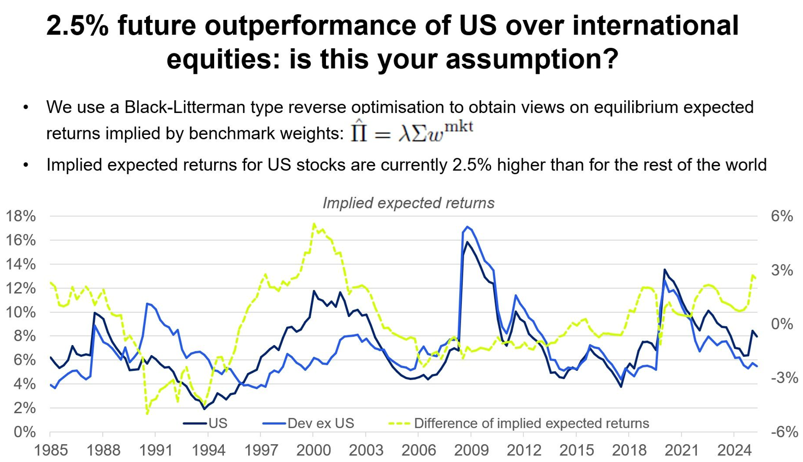
In this sub-section, I will try to reproduce the underlying methodology.

From Figure 2, Goltz³⁷ uses reverse unconstrained mean-variance optimization to compute implied expected returns for U.S. and ex-U.S. equities.

For this, the following pieces of information are needed:

• The universe of assets³⁸

  The MSCI World index will be used as the reference (market capitalization weighted) mean-variance efficient portfolio³⁸ and:

  • The MSCI U.S. index will be used to represent its U.S. equities component
  • The MSCI World ex-USA index will be used to represent its ex-U.S. equities component

• The expected risk free rate

  In the context at hand, the aim is to analyze the difference of implied expected returns between U.S. equities and ex-U.S. equities.

  Hence, there is no need to use an expected risk free rate and it will be set to 0%.

• The vector of the reference mean-variance efficient portfolio weights $w^* \in \mathbb{R}^{2}$

  Because the MSCI World index is used as the reference mean-variance efficient portfolio, the vector of portfolio weights is represented by the vector $w^* = \left( w_{mkt,US}, w_{mkt,ex-US} \right) {}^t$.

  From the MSCI World Index factsheet, the weight of U.S. equities in the MSCI World index is 71.27% on 31st March 2026.

  The corresponding vector of portfolio weights is thus $w^* = \left( 0.7127, 0.2873 \right) {}^t$.

• An estimate of $\Sigma \in \mathcal{M}(\mathbb{R}^{2 \times 2})$, the covariance matrix of the arithmetic returns of the MSCI U.S. index and of the MSCI World ex-USA index, at a one year holding horizon

  Using monthly arithmetic returns³⁹ over the period January 1979 - March 2026 and a simple annualization rule⁴⁰, the empirical covariance matrix $\Sigma$ of these two assets at a one year holding horizon is equal to

  \[\Sigma = \begin{pmatrix} 0.0276 & 0.0179 \\ 0.0179 & 0.0228 \end{pmatrix}\]

• An estimate of the risk tolerance parameter $\lambda$

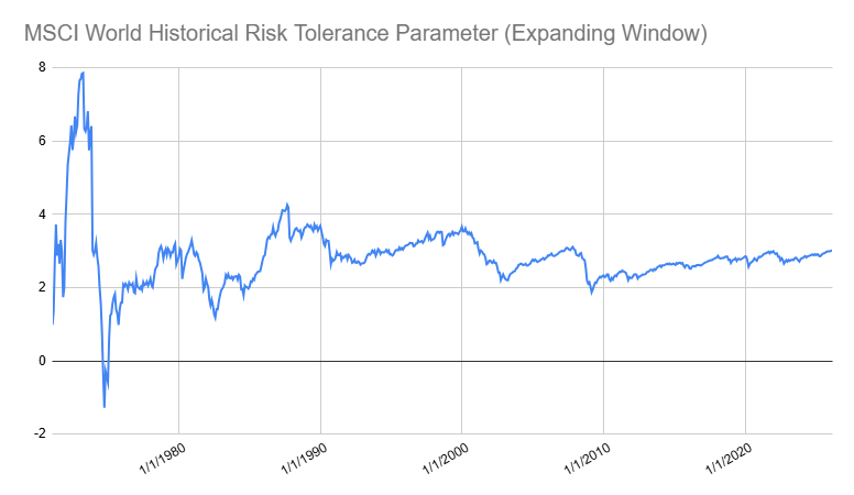
  It is possible to estimate $\lambda$ thanks to the historical risk premium⁴¹ of the MSCI U.S. index over the period January 1979 - March 2026.

  As illustrated in Figure 3, the resulting value of the risk tolerance parameter seems to be around 3.01⁴² on 31st March 2026, even if one needs to be extremely cautious with this kind of historical estimation due to sampling variation²⁴.

  

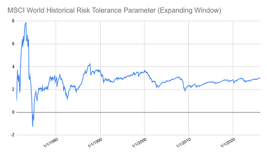
  Figure 3. Historical risk tolerance parameter, MSCI World index, expanding window over the period January 1979 - March 2026.

Thanks to the different estimates above, it is possible to compute the vector of implied expected returns $\mu_{impl} \in \mathbb{R}^{2}$, with $\mu_{impl} = \left( \mu_{impl,US}, \mu_{impl,ex-US} \right) {}^t$, through the formula $ \mu_{impl} = \lambda \Sigma w^* $.

This results in $ \mu_{impl} \approx \left( 7.48\%, 5.82\% \right) {}^t$, which means that investing in the MSCI World index in March 2026 comes with the hidden assumption of an outperformance of U.S. equities over ex-U.S. equities of about 1.7% annualy going forward.

In order to validate the robustness of that conclusion - keeping in mind the remarks in Best and Grauer⁹ - it is also possible to estimate the risk tolerance parameter $\lambda$ using a target annualized expected return of 9.09% for U.S. equities, as reported by Aswath Damodaran at the end of March 2026.

This results in $ \mu_{impl} \approx \left( 9.09\%, 7.07\% \right) {}^t$ and an implied outperformance of U.S. equities over ex-U.S. equities of about 2% annualy going forward.

That figure is closer to Goltz’s³⁷ 2.5%, and since 1.7-2% and 2.5% are in the same ballpark, this validates the methodology detailled above.

How is an investor now supposed to act when presented with that information?

Two possibilities:

• Either he thinks that U.S. equities are indeed likely to outperform ex-U.S. equities by such an amount, in which case he has nothing to do
• Or he thinks that the performance of U.S. equities v.s. ex-U.S. equities might revert to its historical mean⁴³, in which case he might want to decrease his exposure to U.S. equities⁴⁴

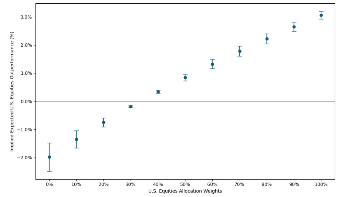
In the later case, he can use Figure 4 as a decision support, for it depicts different possible ranges⁴⁵ of expected annualized outperformance of U.S. equities over ex-U.S. equities as implied by U.S. equities allocation weights.

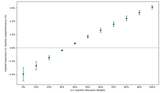
Figure 4. Relative outperformance of U.S. equities over ex‑U.S. equities as implied by U.S. equities allocation weights, annualized expected range.

Incidentally, and maybe contrary to intuition⁴, Figure 4 highlights that neutrality towards U.S. equities outperformance is achieved with an allocation of about only⁴⁶ 35% to U.S. equities…

Conclusion

To sum up this blog post, reverse optimization is a useful method that can help “harness the wisdom of crowds”⁶ and allows to derive the implicit return assumptions of market participants⁶ by exploiting the high predictability of risk, and relying on the plain math of mean-variance optimization⁶.

As usual, feel free to connect with me on LinkedIn or to follow me on Twitter.

–

1. See Herold, U. Computing implied returns in a meaningful way. J Asset Manag 6, 53–64 (2005). ↩ ↩² ↩³ ↩⁴ ↩⁵ ↩⁶ ↩⁷ ↩⁸ ↩⁹ ↩¹⁰ ↩¹¹ ↩¹² ↩¹³ ↩¹⁴ ↩¹⁵ ↩¹⁶ ↩¹⁷ ↩¹⁸ ↩¹⁹ ↩²⁰ ↩²¹ ↩²²

2. See Sharpe, William F., Imputing Expected Security Returns from Portfolio Composition., The Journal of Financial and Quantitative Analysis 9, no. 3 (1974): 463–72. ↩ ↩² ↩³ ↩⁴ ↩⁵ ↩⁶ ↩⁷ ↩⁸ ↩⁹ ↩¹⁰ ↩¹¹ ↩¹² ↩¹³ ↩¹⁴

3. See Al-Thani, Khalifa and Mignacca, Domenico and Steyn, Andries Christiaan and Fusai, Gianluca and Caccioli, Fabio and Germano, G., The Quest for Neutrality in Asset Allocation (November 24, 2025). ↩ ↩² ↩³ ↩⁴

4. See David Ardia, Kris Boudt, Implied Expected Returns and the Choice of a Mean–Variance Efficient Portfolio Proxy, The Journal of Portfolio Management Summer 2015, 41 (4) 68 - 81. ↩ ↩² ↩³ ↩⁴ ↩⁵ ↩⁶ ↩⁷ ↩⁸ ↩⁹ ↩¹⁰ ↩¹¹ ↩¹² ↩¹³

5. Represented by a given list of asset weights and a given covariance matrix. ↩

6. See Two Sigma Client Solutions Team, Estimating Global Investor Views with Reverse Optimization. ↩ ↩² ↩³ ↩⁴ ↩⁵ ↩⁶ ↩⁷ ↩⁸

7. See Ni, X., Malevergne, Y., Sornette, D., Woehrmann, P., 2011. Robust reverse engineering of cross-sectional returns and improved portfolio allocation performance using the CAPM. Journal of Portfolio Management 37 (4), 76–85. ↩ ↩²

8. Sometimes also called the risk aversion parameter, although strictly speaking, the risk aversion is defined as the inverse of the risk tolerance. ↩

9. See Best, M. J., & Grauer, R. R. (1985). Capital Asset Pricing Compatible with Observed Market Value Weights. The Journal of Finance, 40(1), 85–103. ↩ ↩² ↩³ ↩⁴ ↩⁵ ↩⁶ ↩⁷ ↩⁸ ↩⁹

10. The reasoning can be summarized as follows: an hypothetical stock/bond investor needs to increase his stock weight when the risk tolerance $\lambda$ increases due to the budget constraint becoming binding and not because he is more bullish on stocks; in that case, implied expected returns should not vary with $\lambda$. ↩

11. Because the Sharpe Ratio is homogeneous of degree 0, the budget constraint only fixes the scale, so that it is possible to first solve the unconstrained Sharpe Ratio maximization problem and then normalize the obtained optimal portfolio weights. ↩

12. See Markowitz, H.M. (March 1952). Portfolio Selection. The Journal of Finance. 7 (1): 77–91. ↩

13. Bound constraints are sometimes included in inequality constraints for theoretical analysis, but numerically, they are better handled separately. ↩

14. So that binding inequality constraints at optimality are known as well. ↩

15. Because nonnegativity constraints are not binding at optimality. ↩

16. See Dimitris Bertsimas, Vishal Gupta, Ioannis Ch. Paschalidis, (2012) Inverse Optimization: A New Perspective on the Black-Litterman Model. Operations Research 60(6):1389-1403. ↩

17. See Shumway, Tyler and Szefler, Maciej and Yuan, Kathy Zhichao, The Information Content of Revealed Beliefs in Portfolio Holdings (March, 18 2009). ↩ ↩² ↩³ ↩⁴ ↩⁵ ↩⁶ ↩⁷ ↩⁸ ↩⁹ ↩¹⁰ ↩¹¹ ↩¹²

18. See Bevan, A., & Winkelmann, K. (1998). Using the Black-Litterman Global Asset Allocation Model: Three Years of Practical Experience. Fixed Income Research. ↩ ↩² ↩³

19. Which can for example be solved by using simple and exponentially weighted moving average models. ↩

20. See Thomas Idzorek, A step-by-step guide to the Black-Litterman model: Incorporating user-specified confidence levels, Forecasting Expected Returns in the Financial Markets, Academic Press, 2007, Pages 17-38. ↩ ↩²

21. For example, in case the reference mean-variance efficient portfolio is the market portfolio, the portfolio risk premium is by definition equal to the market risk premium. ↩

22. See Satchell, S., Scowcroft, A. A demystification of the Black–Litterman model: Managing quantitative and traditional portfolio construction. J Asset Manag 1, 138–150 (2000). ↩

23. In case of a constant risk free rate, the covariance matrix of the asset arithmetic returns is strictly equal to the covariance matrix of the excess asset arithmetic returns over the risk free rate; in case of a varying risk free rate, though, which is more realistic, the two asset covariance matrices are slighty different from each other but typically not different enough to materially alter any result. ↩ ↩²

24. See Grant, A., Kwon, O.K. & Satchell, S. Properties of risk aversion estimated from portfolio weights. J Asset Manag 25, 427–444 (2024). ↩ ↩²

25. See Partridge, L. and Croce, R., 2012. Risk Parity for the Long Run. ↩

26. See for example Envestnet Capital Markets Assumptions Methodology, 2023. ↩

27. Or, more generally, to use a/the forecast range as the target upper, lower, and central⁶ implied expected return for that asset. ↩ ↩²

28. See Damodaran, Aswath, Equity Risk Premiums (ERP): Determinants, Estimation and Implications - The 2023 Edition. ↩

29. See Robert C. Merton. On Estimating the Expected Return on the Market: An Exploratory Investigation. Journal of Financial Economics 8 (December 1980), 323-61. ↩

30. Unlike the risk tolerance parameter, there exists no sensible fixed value³⁰ for the Lagrange multiplier $\gamma$; attempts to circumvene that problem have been made, c.f. for example Xin and Ding³¹, but they are still relatively impractical. ↩

31. See Xin, L., Ding, S. Expected returns with leverage constraints and target returns. J Asset Manag 22, 200–208 (2021). ↩ ↩²

32. See Allaj, E. (2020). The Black–Litterman model and views from a reverse optimization procedure: An out-of-sample performance evaluation. Computational Management Science, 17(3), 465-492. ↩ ↩²

33. Called the dual problem of mean-variance optimization in Shumway et al.¹⁷. ↩

34. See P. Jorion, Bayes-Stein estimation for portfolio analysis, Journal of Financial and Quantitative Analysis 21 (3) (1986) 279–292. ↩

35. See C. Wang, T. Tong, L. Cao, B. Miao, Non-parametric shrinkage mean estimation for quadratic loss functions with unknown covariance matrices, Journal of Multivariate Analysis 125 (2014) 222–232. ↩

36. See Levy, M., and Roll, R. The Market Portfolio may be Mean-Variance Efficient After All. Review of Financial Studies, 23 (2010), pp. 2464-2461. ↩

37. See Felix Goltz, LinkedIn post. ↩ ↩² ↩³ ↩⁴ ↩⁵

38. All indexes are Gross Total Return and denominated in USD. ↩ ↩²

39. To be noted that, like for the expected risk free rate set to 0%, there is no need either to use asset historical excess arithmetic returns for the computation of $\Sigma$ - raw historical arithmetic returns are perfectly fine since we are not computing implied excess expected returns but implied expected returns. ↩

40. Multiplication of the monthly covariance matrix by 12. ↩

41. The U.S. historical monthly risk free rate has been taken from the Fama and French data library. ↩

42. The exact value used 3.015222148. ↩

43. See Marin Lolic, Robert Panariello, Som Priestley, Validating Your U.S. and Non-U.S. Equity Exposure, T. ROWE PRICE INSIGHTS, February 2023. ↩

44. An investor in a MSCI World ETF cannot directly decrease his exposure to U.S. equities, but there are at least two solutions: either keep the MSCI World ETF and buy an additional MSCI World ex-US ETF or fully replace the MSCI World ETF by a U.S. equities ETF and a MSCI World ex-US ETF. ↩

45. The ranges have been computed using the two procedures to estimate the risk tolerance parameter $\lambda$ already used to compute the 1.7-2% range in case the U.S. equities allocation weight was fixed to 71.27%; another possibility would be to use different risk tolerance parameters, for example 2 and 4, as suggested by Figure 3. ↩

46. And not 50% for example. ↩