Capital Market Assumptions: Combining Institutions’ Forecasts for Improved Accuracy
Capital market assumptions1 (CMAs) are forecasts of future risk/return characteristics for broad asset classes over the next 5 to 20 years produced by leading investment managers, consultants and advisors2.
These forecasts are well-reasoned, analytically rigorous assumptions about uncertain future market movements2 and are used almost universally among institutional investors2, for example as inputs to their stategical asset allocation3.
In this blog post, I will show that combining capital market assumptions might be preferable to using any institution-specific estimates and I will describe a couple of practical data issues encountered when doing so.
The variability of capital market assumptions
Each year since 2010, people at Horizon Actuarial ask different investment firms to provide their capital market assumptions4, and release an associated survey.
Figure 1 - taken from the 2023 edition of that survey4 - clearly shows significant differences in expected returns and standard deviations among investment advisors4.
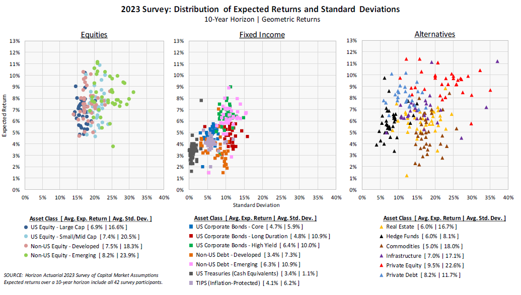
Of course, variability should come as no surprise, because different institutions use different forecasting methodologies and/or have different views on the future5…
Nevertheless, such a high variability is definitely an issue for an investor since it is impossible to identify a priori the institution that will produce the most accurate forecasts of future returns, standard deviations and correlations.
The risk of relying on a “bad” institution for an investor is therefore very real…
Combining capital market assumptions
The general forecast combination problem
The specific problem described in the previous section is an instance of a more general problem known as the forecast combination problem, introduced as follows by Timmermann6:
Faced with multiple forecasts of the same variable, an issue that immediately arises is how best to exploit information in the individual forecasts. In particular, should a single dominant forecast be identified or should a combination of the underlying forecasts be used to produce a pooled summary measure?
From the forecasting literature, a pragmatic solution to this problem is to average all individual forecasts, which leads to an equal-weighting forecast combination scheme.
While guaranteed to degrade the forecast accuracy v.s. using the “best” individual forecast7, such a forecast combination scheme has repeatedly been found to outperform sophisticated adaptive combination methods in empirical applications6, thus setting a benchmark that has proved surprisingly difficult to beat6.
As an interesting side note for readers of this blog, it turns out that the forecast combination problem is closely related to the mean-variance portfolio optimization problem6.
Averaging capital market assumptions
From a theoretical perspective, an equal-weighted forecast combination scheme is well-suited to the specific context of capital market assumptions.
Indeed, given the significant effort, resources and intellectual capital [put] into the production of [capital market assumptions]2, it is reasonable to assume that the relative size of the variance of the forecast errors associated with [the] different forecasting methods6 are all similar, which in theory favors an equal-weighting forecast combination scheme6.
From a practical perspective, an equal-weighted forecast combination scheme is easy to compute and does not introduce any parameter estimation errors, which are known to be a serious problem for many combination techniques6.
As for the forecast accuracy of that scheme, it is possible to have an idea of it thanks to Figure 2 - taken from Sebastian2 -, which compares:
- The min-max range of 10-year capital market assumptions produced by 19 investment firms for misc. asset classes in 2013
- The associated averaged 10-year capital market assumptions
- The subsequent realized 10-year returns
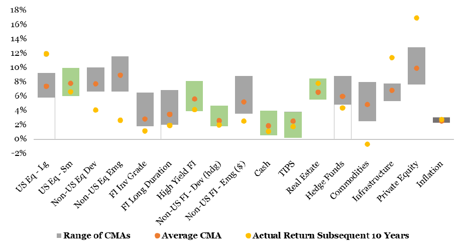
From Figure 2, it is visible that:
-
Using averaged capital market assumptions v.s. firm-specific estimates prevented8 severe over/under-predictions for a couple of asset classes, like a ~3% over-prediction for Emerging Markets equities, which is great.
-
In the majority of cases, the average capital market assumption [is] an unreliable guide to the future return2, which is not so great, but which ultimately depends on the accuracy and/or bias of the individual capital market assumptions and not on the forecast combination scheme itself9.
That being said, a sample size of 1 observation per asset class is anyway maybe a little too small for reaching definite conclusions…
Capital market assumptions data preparation
Before being able to average capital market assumptions originating from different institutions, it is first required to collect and normalize these forecasts.
Below are examples of typical data preparation steps for doing so.
Collecting a sufficient number of forecasts
Figure 3 - taken from an ECR Research report10 - illustrates the variety of forecast horizons for which a representative sample of leading investment firms provide their capital market assumptions.
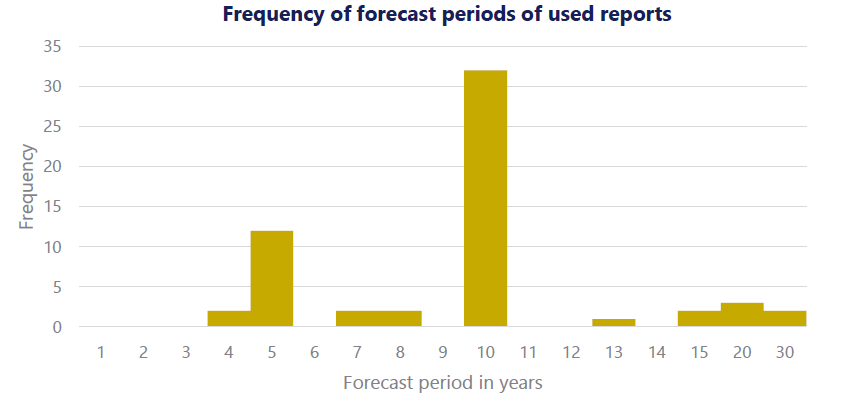
From Figure 3, and in oder to combine as many distinct capital market assumptions as possible, it seems a good idea to focus on collecting forecasts for either a 5-year or a 10-year horizon, with a preference for a 10-year horizon.
Reconciliating asset classes across institutions
Because not all investment advisors use the same asset classes when developing their capital market assumptions4, reconciliating different asset classes across institutions is mandatory and requires to exercice judgment in classifying [institutions] capital market assumptions into a standard set of asset2.
As a side note, there are also sometimes inconsistencies in the name of asset classes.
For example, under the asset class label Developed Equities, different institutions might mean:
- An asset class represented by the MSCI World Index, which would be the standard convention
- An asset class represented by the MSCI World ex-US Index
- An asset class represnted by the MSCI EAFE Index
Converting expected returns
Converting real expected returns to nominal expected returns
The vast majority of institutions provide expected returns in nominal terms, but a couple of them provide expected returns in real terms.
In order to compare apples to apples, it is necessary to convert these real returns into nominal returns by adding local expected inflation11, that is:
- U.S. expected inflation, for U.S. asset classes (U.S. Equities, U.S. Bonds…) as well as usually for commodities
- Eurozone expected inflation12, for euro-denominated asset classes (E.M.U. Equities, EUR Bonds…)
- Emerging countries inflation12, for Emerging Equities
- …
Converting expected returns currencies
Depending on the institution and on the asset class, expected returns can be provided in:
- USD, or another investable currency like EUR
- USD EUR-hedged, or another investable currency pair hedged like EUR JPY-hedged
- Local currency
- Local currency investable currency-hedged, or investable currency local currency-hedged or whatever weird combination
In order to again compare apples to apples, it is necessary to convert all the currencies appearing in the different expected returns into a unique investable currency.
Converting expected returns in an investable currency to expected returns in another investable currency
The most usual scenario is the need to convert expected returns initially provided in an investable currency like USD into another investable currency like EUR.
This convertion - ignoring the small geometric interaction11 - is done by adding the expected foreign exchange return to the expected returns11.
Converting investable currency-hedged expected returns to investable currency-unhedged expected returns
Expected returns for “foreign” fixed income asset classes are frequently provided as “foreign currency”-hedged13.
The convertion from “foreign currency”-hedged expected returns to “foreign currency”-unhedged expected returns is done by correcting for the expected nominal risk-free rate differential14, that is, by adding the difference between the foreign and the local cash returns.
Converting expected returns in local currency to expected returns in an investable currency
Many institutions provide expected returns in local currency to avoid the issue of [determining] what an asset’s expected return will be from a particular investor’s currency perspective13.
Ultimately, though, an investor needs to make a currency decision, and expected returns in local currency must be converted into expected returns in an investable currency like USD or EUR.
For single-currency asset classes, like U.S. Equities or Eurozone Government Bonds, this is not an issue, c.f. the previous sub-sections.
For multi-currency asset classes, like Emerging Market Equities or Global Government Bonds, the situation is more complex because a proper conversion would at the very least require assumptions on:
- The expected currency weights in the asset class at the forecast horizon
- The expected foreign exchange return at the forecast horizon, for all currencies
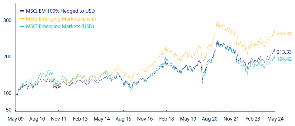
To be noted that ignoring this complexity is probably not an option, as illustrated in Figure 4 - taken from the factsheet of the MSCI Emerging Markets Index -, which shows a ~3% difference in annualized returns over the last 10 years between the “local currency” and the “USD” flavors of the MSCI Emerging Markets Index.
Between those two extremes, finding a pragmatic solution depending on the exact asset class is the best thing to do!
Other convertions
The need for other weird currency convertions might be encountered, at which point a balance must be struck between:
- Adding new forecasts, possibly unique, to the list of collected capital market assumptions
- Adding complexity to the capital market assumptions collection process
Converting geometric expected returns to arithmetic expected returns
Nearly all institutions produce estimates of geometric (compound) asset class returns14, while standard mean-variance portfolio optimization15 requires expected returns to be provided in arithmetic rather than in geometric terms14.
In order to approximately convert geometric expected returns to arithmetic expected returns, it suffices to add half of the expected asset class variance11.
As a down-to-earth comment on why is that, I cannot resist sharing what people at Verus wrote in the 2024 edition of their capital market assumptions:
This is the industry standard approach, but requires a complex explanation only a heavy quant could love, so we have chosen not to provide further details in this document […]
Converting expected standard deviations/correlations
Similar to expected returns, expected standard deviations and correlations should also be converted into an investor’s chosen currency.
Unfortunately, this conversion is far more complex to perform than that of expected returns, so that - unless specified otherwise by the originating institution - it is probably best to leave the original expected standard deviations and correlations untouched.
Implementations
Implementation in Portfolio Optimizer
Portfolio Optimizer allows to retrieve minimum, maximum and averaged 10-year capital market assumptions (nominal arithmetic and geometric returns, standard deviations, correlations) from leading financial institutions and for selected asset classes:
- In EUR, through the endpoint
/markets/capital-assumptions/eur - In USD, through the endpoint
/markets/capital-assumptions/usd
A couple of remarks:
-
The list of financial institutions from which capital market assumptions have been sourced is provided in output of these endpoints.
-
The supported asset classes, together with a representative benchmark, are the following:
Asset Class Asset Class Label in Portfolio Optimizer Representative Benchmark U.S. Cash cash-us J.P. Morgan Cash Index USD Eurozone Cash cash-eurozone J.P. Morgan Cash Index Euro Currency U.S. Government Bonds governmentBonds-us Bloomberg U.S. Treasury Index Eurozone Government Bonds governmentBonds-eurozone Bloomberg Euro Aggregate Treasury Index U.S. Investment Grade Corporate Bonds corporateBonds-us ICE BofA US Corporate Index Eurozone Investment Grade Corporate Bonds corporateBonds-eurozone ICE BofA Euro Corporate Index U.S. Equities equities-us MSCI USA Index Eurozone Equities equities-eurozone MSCI EMU Index Developed Markets Equities equities-developedMarkets MSCI Developed Markets Index Emerging Markets Equities equities-emergingMarkets MSCI Emerging Markets Index Commodities commodities-all Bloomberg Commodity Index Gold gold-all Gold Spot Price -
The expected correlation matrices provided in output of these endpoints are not guaranteed to be complete nor valid.
- In case a correlation matrix is complete but invalid, it is possible to compute its nearest valid correlation matrix thanks to the endpoint
/assets/correlation/matrix/nearest - In case a correlation matrix is incomplete, Portfolio Optimizer provides no solution for now but stay tuned!
- In case a correlation matrix is complete but invalid, it is possible to compute its nearest valid correlation matrix thanks to the endpoint
Last, if you would like a specific currency or a specific asset class to be integrated into Portfolio Optimizer, feel free to reach out.
Implementations elsewhere
I am aware of other capital market assumptions “averaging” services as described in this blog post:
- Horizon Actuarial yearly survey of capital market assumptions
- Peresec interactive summary of long-term capital market assumptions
- ECR Research strategic asset allocation quarterly reports
Conclusion
This concludes this first blog post on capital market assumptions.
As usual, feel free to connect with me on LinkedIn or to follow me on Twitter.
–
-
Or capital market expectations (CMEs). ↩
-
See Sebastian, Michael D., The Accuracy and Use of Capital Market Assumptions. ↩ ↩2 ↩3 ↩4 ↩5 ↩6 ↩7
-
See Research Affiliates Capital Market Expectations Methodology, 05.31.2023. ↩
-
See Horizon Actuarial Services LLC, Survey of Capital Market Assumptions, 2023 Edition. ↩ ↩2 ↩3 ↩4
-
Additionally, Horizon Actuarial4 notes that different institutions publish their capital market assumptions at different dates. ↩
-
See Allan Timmermann, Chapter 4 Forecast Combinations, Editor(s): G. Elliott, C.W.J. Granger, A. Timmermann, Handbook of Economic Forecasting, Elsevier, Volume 1, 2006, Pages 135-196. ↩ ↩2 ↩3 ↩4 ↩5 ↩6 ↩7
-
Again, impossible to identify ex-ante. ↩
-
Of course, Figure 2 also shows that using averaged capital market assumptions prevented to use the best firm-specific estimates, but as discussed in the previous section, it is impossible to identify these ex-ante, so that’s not a real drawback. ↩
-
One could think of using an optimal-weighting forecast combination scheme, with for example the objective of minimizing the out-of-sample forecast error, but due to the small sample size over which the optimal weights would need to be estimated, such a scheme would probably lead to poor performance v.s. an equal-weighting scheme, as is usual in the forecasting litterature, c.f. Timmermann6. ↩
-
See Lai Hoang, Ummul Ruthbah, Long-Term Capital Market Assumptions Public Equities. ↩ ↩2 ↩3 ↩4
-
With or without an appropriate weighting per country representative of the asset class weighting per country, which quickly becomes a mess to manage… ↩ ↩2
-
See BNP Paribas AM, Long-Term Asset Allocation - The slow return to normal, Portfolio perspectives, White paper. ↩ ↩2
-
See Invesco, 2024 long-term capital market assumptions. ↩ ↩2 ↩3
-
The same remark also applies to other portfolio allocation or optimization techniques, like Monte Carlo simulations. ↩