From Volatility Forecasting to Covariance Matrix Forecasting: The Return of Simple and Exponentially Weighted Moving Average Models

In the initial post of the series on volatility forecasting, I described the simple and the exponentially weighted moving average forecasting models, that are both easy to understand and relatively performant in practice.

Beyond (univariate) volatility forecasting, these two models are also widely used in (multivariate) covariance matrix forecasting¹²³, for the very same reasons.

In this blog post, I will detail the simple and exponentially weighted moving average covariance matrix forecasting models and I will illustrate their empirical performances in the context of monthly covariance matrix forecasting for a multi-asset class ETF portfolio.

Mathematical preliminaries

Covariance matrix modelling

Let $n$ be the number of assets in a universe of assets and $r_t \in \mathbb{R}^n$ be the vector of the (logarithmic) return of these assets over a time period $t$.

In all generality, $r_t$ can be expressed as²

\[r_t = \mu_t + \epsilon_t\]

, where:

• $\mu_t \in \mathbb{R}^n$, $\mu_t = \mathbb{E} \left[ r_t \right]$, is a predictable quantity representing the vector of the (conditional) assets mean return over the time period $t$
• $\epsilon_t \in \mathbb{R}^n$, $\epsilon_t = r_t - \mathbb{E} \left[ r_t \right]$, is an unpredictable error term, often referred to as a vector of “shocks” or as a vector of “random disturbances”², over the time period $t$

The asset (conditional) covariance matrix $\Sigma_t \in \mathcal{M}(\mathbb{R}^{n \times n})$ is then defined by¹

\[\begin{aligned} \Sigma_t &= Cov \left[ r_t \right] \\ &= \mathbb{E} \left[ \left( r_t - \mu_t \right) \left( r_t - \mu_t \right) {}^t \right] \\ &= \mathbb{E} \left[ r_t r_t {}^t \right] - \mathbb{E} \left[ r_t \right] \mathbb{E} \left[ r_t \right] {}^t \\ &= \mathbb{E} \left[ r_t r_t {}^t \right] - \mu_t \mu_t {}^t \\ \end{aligned}\]

From this general model for asset returns, it is possible to derive different models for the asset covariance matrix depending on working assumptions.

In this blog post, the main working assumption will be that the assets mean return over any of the considered time periods $t$ is zero, that is, $\mu_t = 0_n$.

From a previous blog post, such an assumption is routinely made when working with daily stock returns but is also empirically justified when working with lower frequency data on a wide range of assets.

Indeed, as highlighted by Johansson et al.²

[…] the mean [$\mu_t$] is small enough […] for most daily, weekly, or monthly stock, bond, and futures returns, factor returns, and index returns.

Covariance proxies

Under the working assumption of the previous sub-section, the covariance matrix $\Sigma_t$ is then equal⁴ to the second moment $\mathbb{E} \left[ r_t r_t {}^t \right]$.

As a consequence, the outer product of the asset returns $ r_t r_t {}^t $ over a time period $t$ (a day, a week, a month..) is a covariance estimate $\tilde{\Sigma}_t$ - or covariance proxy⁵ - for the asset returns covariance matrix over the considered time period.

To be noted that other covariance proxies exist, like realized covariances⁵ or asset regularized returns⁶, but they will not be discussed in this blog post.

Correlation matrix modelling

The asset (conditional) correlation matrix $C_t \in \mathcal{M}(\mathbb{R}^{n \times n})$ is related to the asset covariance matrix $\Sigma_t$ through the standard formula⁷:

\[C_t = V_t^{-1} \Sigma_t V_t^{-1}\]

, where $V_t \in \mathcal{M}(\mathbb{R}^{n \times n})$ is the diagonal matrix of the asset standard deviations

\[V_t = \begin{pmatrix} \sqrt {\left(\Sigma_t\right)_{1,1}} & 0 & ... & 0 \\ 0 & \sqrt {\left(\Sigma_t\right)_{2,2}} & ... & 0 \\ ... & ... & ... & ... \\ 0 & 0 & ... & \sqrt {\left(\Sigma_t\right)_{n,n}} \end{pmatrix}\]

Simple moving average covariance matrix forecasting model

The simple moving average (SMA) covariance matrix forecasting model⁸, also known as the rolling historical covariance matrix forecasting model², uses an equally weighted moving average [of covariance proxies] calculated on a […] data window [of fixed size $k \geq 1$] that is rolled over time² in order to forecast the asset returns covariance matrix over a time period $t$.

Forecasting formulas

Under a simple moving average covariance matrix forecasting model, forecasting formulas are:

• To estimate the next period’s asset returns covariance/correlation matrix:

  \[\hat{\Sigma}_{T+1} = \frac{1}{k} \sum_{i=1}^{k} \tilde{\Sigma}_{T+1-i}\] \[\hat{C}_{T+1} = \hat{V}_{T+1}^{-1} \hat{\Sigma}_{T+1} \hat{V}_{T+1}^{-1}\]

• To estimate the next $h$-period’s ahead asset returns covariance/correlation matrix, $h \geq 2$:

  \[\hat{\Sigma}_{T+h} = \frac{1}{k} \left( \sum_{i=1}^{k-h+1} \tilde{\Sigma}_{T+1-i} + \sum_{i=1}^{h-1} \hat{\Sigma}_{T+h-i} \right)\] \[\hat{C}_{T+h} = \hat{V}_{T+h}^{-1} \hat{\Sigma}_{T+h} \hat{V}_{T+h}^{-1}\]

• To estimate the averaged asset returns covariance/correlation matrix⁶ over the next $h$ periods:

  \[\hat{\Sigma}_{T+1:T+h} = \frac{1}{h} \sum_{i=1}^{h} \hat{\Sigma}_{T+i}\] \[\hat{C}_{T+1:T+h} = \frac{1}{h} \sum_{i=1}^{h} \hat{C}_{T+i}\]

Specific cases

The simple moving average covariance matrix forecasting model encompasses two specific models:

• The random walk model, which corresponds to $k = 1$.

  Under this model, the forecast of the next period’s asset returns covariance matrix is the current period’s asset returns covariance matrix.

• The historical average model, which corresponds to $k = T$.

  Under this model, the forecast of the next period’s asset returns covariance matrix is the long term average of the past periods’ asset returns covariance matrix.

How to choose the window size?

Like for its univariate couterpart, selecting the “best” window size $k$ of a simple moving average covariance matrix forecasting model is a problem in itself, c.f. the associated blog post.

In addition, and this time specific to the multivariate nature of that forecasting model, the rolling window covariance estimate is not full rank¹ when $k < n$, so that specific post-processing might need to be implemented in order to ensure that covariance matrix forecasts are positive definite⁹.

Exponentially weighted moving average covariance matrix forecasting model

Menchero and Morozov¹⁰ notes that:

If return distributions were stationary, then using the maximum sample size and equally weighting every observation [- that is, using an historical average forecasting model, c.f. the previous section -] would minimize sampling error and hence produce the most accurate forecasts. Return distributions, however, are not stationary. Events that occurred 10 years ago have little to do with current [ones]. Therefore, to reflect current market conditions, we must give more weight to recent observations.

This remark leads to the introduction of the exponentially weighted moving average (EWMA) covariance matrix forecasting model⁸, which, thanks to a decay factor $\lambda \in [0, 1]$, gives $\lambda$-exponentially less emphasis to distant past covariance proxies v.s. more recent ones in order to forecast the asset returns covariance matrix over a time period $t$¹¹.

Incidentally, the exponentially weighted moving average covariance matrix forecasting model is perhaps the most widely used […] model among practitioners¹², in particular due
to its use in the RiskMetrics VaR software of J.P. Morgan¹².

Forecasting formulas

Under an exponentially weighted moving average covariance matrix forecasting model, forecasting formulas are:

• To estimate the next period’s asset returns covariance/correlation matrix:

  \[\hat{\Sigma}_{T+1} = \frac{1 - \lambda}{1 - \lambda^{T}} \sum_{i=1}^{T} \lambda^{T-i} \tilde{\Sigma}_{i}\] \[\hat{C}_{T+1} = \hat{V}_{T+1}^{-1} \hat{\Sigma}_{T+1} \hat{V}_{T+1}^{-1}\]

• To estimate the next $h$-period’s ahead asset returns covariance/correlation matrix, $h \geq 2$:

  \[\hat{\Sigma}_{T+h} = \hat{\Sigma}_{T+1}\] \[\hat{C}_{T+h} = \hat{C}_{T+1}\]

  This result means that covariance and correlation matrix forecasts beyond the (immediate) next period are all equal to the covariance and correlation matrix forecast for that next period, in a kind of random walk model way, and is a known limitation of this model when multi-period ahead forecasts are required.

• To estimate the averaged asset returns covariance/correlation matrix⁶ over the next $h$ periods:

  \[\hat{\Sigma}_{T+1:T+h} = \frac{1}{h} \sum_{i=1}^{h} \hat{\Sigma}_{T+i} = \hat{\Sigma}_{T+1}\] \[\hat{C}_{T+1:T+h} = \frac{1}{h} \sum_{i=1}^{h} \hat{C}_{T+i} = \hat{C}_{T+1}\]

How to choose the decay factor?

Like its univariate couterpart, there are essentially two¹³ procedures to choose the decay factor $\lambda$ of an exponentially weighted moving average covariance matrix forecasting model:

• Using recommended values from the literature (0.94, 0.97…).

• Determining the optimal value w.r.t. the forecast horizon $h$, for example through the minimization of the root mean square error (RMSE) between the forecasted covariance matrix over the desired horizon and the observed covariance matrix over that horizon¹³.

C.f. the the associated blog post for more details.

Implementation in Portfolio Optimizer

Portfolio Optimizer implements:

• The simple moving average covariance and correlation matrix forecasting model through the endpoints /assets/covariance/matrix/forecast/sma and /assets/correlation/matrix/forecast/sma
• The exponentially weighted moving average covariance and correlation matrix forecasting model through the endpoints /assets/covariance/matrix/ewma and /assets/correlation/matrix/forecast/ewma

All these endpoints support the 2 covariance proxies below:

• Squared (close-to-close) returns
• Demeaned squared (close-to-close) returns

The second group of endpoints allows to automatically determine the optimal value of its parameter (the decay factor $\lambda$) using a proprietary variation of the procedures described in the RiskMetrics technical document¹⁴.

Example of usage - Covariance matrix forecasting at monthly level for a portfolio of various ETFs

As an example of usage, I propose to evaluate the empirical performances of the simple and exponentially weighted moving average covariance matrix forecasting models in the context of a portfolio of 10 ETFs representative¹⁵ of misc. asset classes:

• U.S. stocks (SPY ETF)
• European stocks (EZU ETF)
• Japanese stocks (EWJ ETF)
• Emerging markets stocks (EEM ETF)
• U.S. REITs (VNQ ETF)
• International REITs (RWX ETF)
• U.S. 7-10 year Treasuries (IEF ETF)
• U.S. 20+ year Treasuries (TLT ETF)
• Commodities (DBC ETF)
• Gold (GLD ETF)

Methodology

At the end of each month, I will compare the (averaged) covariance matrix forecasts produced by the simple and exponentially weighted moving average covariance matrix forecasting models¹⁶ at a one-month horizon to the next month’s empirical covariance matrix.

The performance criterion considered will be the mean squared error (MSE) between the forecasted and the observed covariance matrices, which is a direct¹⁷ method to evaluate the out-of-sample forecast accuracy of a covariance matrix forecasting model, c.f. for example in Johansson et al.¹

Results

Results over the period 31st January 2008 - 31st July 2023¹⁸ are the following¹⁹, with a graphical illustration on Figure 1:

Covariance matrix model	Covariance matrix MSE
SMA, window size of all the previous months (historical average model)	9.59 $10^{-6}$
SMA, window size of the previous year	9.08 $10^{-6}$
EWMA, optimal $\lambda$20	6.52 $10^{-6}$
EWMA, $\lambda = 0.97$	6.37 $10^{-6}$
SMA, window size of the previous month (random walk model)	6.06 $10^{-6}$
EWMA, $\lambda = 0.94$	5.78 $10^{-6}$

Figure 1. Next month's covariance matrix forecasting model MSE, 10-ETF universe, 31st January 2008 - 31st July 2023.

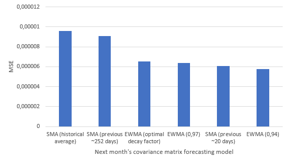
A couple of general remarks from Figure 1:

• Both covariance matrix forecasting models seem to do an excellent job at forecasting next month’s empirical covariance matrix; unfortunately, the very low MSEs are misleading - more on this in the next sub-section.
• The exponentially weighted moving average covariance matrix forecasting model is generally more performant than the simple moving average covariance matrix forecasting model - provided a proper decay factor is used - which is consistent with the higher reactivity of that model.
• There is a penalty to pay in terms of MSE for automatically determining the optimal decay factor of the exponentially weighted moving average covariance matrix forecasting model v.s. using a pre-defined value.

Results, take 2

Because a covariance matrix depends on both asset variances and correlations, let’s have a look at the MSE²¹ between the forecasted and the observed correlation matrices associated to the covariance matrices of the previous sub-section, with a graphical illustration on Figure 2:

Covariance matrix model	Correlation matrix MSE
SMA, window size of the previous month (random walk model)	8.19
SMA, window size of all the previous months (historical average model)	8.10
EWMA, $\lambda = 0.94$	7.67
SMA, window size of the previous year	6.50
EWMA, $\lambda = 0.97$	6.36
EWMA, optimal $\lambda$20	5.87

Figure 2. Next month's correlation matrix forecasting model MSE, 10-ETF universe, 31st January 2008 - 31st July 2023.

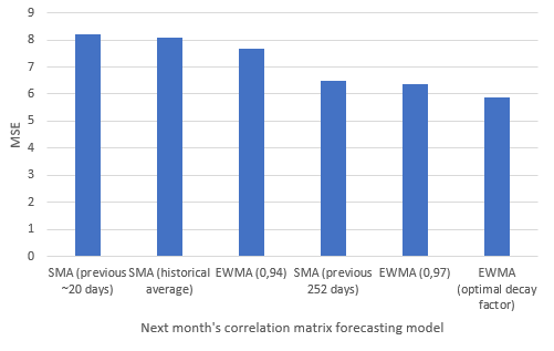
It appears that the correlation matrix forecasts are actually pretty bad, or at the very least, not as good as the covariance matrix forecasts MSEs have led us to believe in the previous sub-section!

The explanation is that the covariance matrix forecasts MSEs are artificially deflated due to the difference in scale²² between asset returns variances and correlations, so that they are more indicative of the quality of the variances forecasts than of the correlations forecasts…

Question is then, how bad are the correlation matrix forecasts?

Figure 3²¹ illustrates the MSEs obtained when forecasting the next month’s correlation matrix by the observed next month’s correlation matrix randomly perturbed by a given noise level.

Figure 3. Next month's correlation matrix perturbation level v.s. resulting MSE, 10-ETF universe, 31st January 2008 - 31st July 2023.

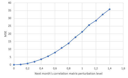
Figure 3 is interpreted as follows:

• When all the correlation coefficients of the forecasted next month’s correlation matrix are equal to those of the observed next month’s correlation matrix (perturbation level equal to 0), the resulting MSE is 0.
• When all the correlation coefficients of the forecasted next month’s correlation matrix are within $\pm 1.4$ from those of the observed next month’s correlation matrix (perturbation level equal to 1.4), the resulting MSE is ~35.

Reverse-reading Figure 3, it is thus possible to conclude that:

• The correlation coefficients forecasted by the worst performing covariance forecasting model (MSE ~8.19) are on average within $\pm 0.60$ of the observed correlation coefficients.
• The correlation coefficients forecasted by the best performing covariance forecasting model (MSE ~5.87) are on average within $\pm 0.50$ of the observed correlation coefficients.

So, all in all, the correlation matrix forecasts produced by the simple and exponentially weighted moving average covariance matrix forecasting models are not that bad, but an average $\pm 0.50$ or $\pm 0.60$ uncertainty around the forecasted correlations would definitely gain to be improved.

As a final remark here, one should always be wary of covariance matrix forecasting results reported in terms of “covariance” MSEs…

Conclusion

This first blog post on covariance matrix forecasting introduced two baseline models, which are direct extensions of volatility forecasting models.

The observed discrepencies between those models’ covariance and correlation matrix forecasting performances lead to wonder whether it is possible to improve these models by separating the covariance matrix forecasting process into two steps - a first volatility forecasting step and a second correlation matrix forecasting step.

This will be the subject of the next blog post in this series.

Meanwhile, feel free to connect with me on LinkedIn or to follow me on Twitter.

–

1. See Kasper Johansson, Mehmet G. Ogut, Markus Pelger, Thomas Schmelzer and Stephen Boyd (2023), A Simple Method for Predicting Covariance Matrices of Financial Returns, Foundations and Trends in Econometrics: Vol. 12: No. 4, pp 324-407. ↩ ↩² ↩³ ↩⁴

2. See Valeriy Zakamulin, A Test of Covariance-Matrix Forecasting Methods, The Journal of Portfolio Management Spring 2015, 41 (3) 97-108. ↩ ↩² ↩³ ↩⁴ ↩⁵ ↩⁶

3. See Guijarro-Ordonez, Jorge and van Beek, Misha and Dhaliwal, Amandeep, A Simple Responsive Covariance Matrix Forecaster for Multiple Horizons and Asset Classes. ↩

4. Or at least, should be well approximated by that second moment… ↩

5. See Patton, A.J., Sheppard, K. (2009). Evaluating Volatility and Correlation Forecasts. In: Mikosch, T., Kreiß, JP., Davis, R., Andersen, T. (eds) Handbook of Financial Time Series. Springer, Berlin, Heidelberg. ↩ ↩²

6. See Gianluca De Nard, Robert F. Engle, Olivier Ledoit, Michael Wolf, Large dynamic covariance matrices: Enhancements based on intraday data, Journal of Banking & Finance, Volume 138, 2022, 106426. ↩ ↩² ↩³

7. See Wikipedia, Covariance matrix. ↩

8. This covariance matrix forecasting model is a direct extension of its volatility forecasting model counterpart. ↩ ↩²

9. In all generality, specific post-processing might anyway need to be implemented to ensure that covariance matrix forecasts are well-conditioned, c.f. Johansson et al.¹ ↩

10. See Jose Menchero, Andrei Morozov, Improving Risk Forecasts Through Cross-Sectional Observations, The Journal of Portfolio Management Spring 2015, 41 (3) 84-96. ↩

11. The exponentially weighted moving average covariance matrix forecasting model is a special case of the diagonal vec multivariate GARCH model of Engle and Kroner²³, and corresponds to an integrated GARCH model with no constant vector¹². ↩

12. See Richard D.F. Harris, Fatih Yilmaz, Estimation of the conditional variance–covariance matrix of returns using the intraday range, International Journal of Forecasting, Volume 26, Issue 1, 2010, Pages 180-194. ↩ ↩² ↩³

13. Other procedures are described in the RiskMetrics technical document¹⁴. ↩ ↩²

14. See RiskMetrics. Technical Document, J.P.Morgan/Reuters, New York, 1996. Fourth Edition. ↩ ↩²

15. These ETFs are used in the Adaptative Asset Allocation strategy from ReSolve Asset Management, described in the paper Adaptive Asset Allocation: A Primer²⁴. ↩

16. As implemented in Portfolio Optimizer. ↩

17. Direct methods use a proxy for the true covariance matrix to evaluate the predictor, while indirect methods use the covariance predictor on tasks of interest, such as portfolio construction or portfolio tracking¹. ↩

18. (Adjusted) daily prices have have been retrieved using Tiingo. ↩

19. Using the outer product of asset returns - assuming a mean return of 0 - as covariance proxy, and using an expanding historical window of asset returns. ↩

20. The optimal decay factor $\lambda$ is computed at the end of every month using all the available asset returns history up to that point in time, as implemented in Portfolio Optimizer; thus, there is no look-ahead bias. ↩ ↩²

21. The maximum perturbation level on Figure 3 is limited to 1.4, because that level correponds to the MSE also reached by forecasting next month’s correlation matrix by a random correlation matrix; so, there is no practical interest in going beyond that level up to the theoretical limit of 2. ↩ ↩²

22. Especially for the variance of daily asset returns, as is the case here. ↩

23. See Engle RF, Kroner KF. Multivariate Simultaneous Generalized ARCH. Econometric Theory. 1995;11(1):122-150. ↩

24. See Butler, Adam and Philbrick, Mike and Gordillo, Rodrigo and Varadi, David, Adaptive Asset Allocation: A Primer. ↩