Correlation Matrix Stress Testing: Random Perturbations of a Correlation Matrix

In the previous posts of this series, I detailed a methodology to perform stress tests on a correlation matrix by linearly shrinking a baseline correlation matrix toward an equicorrelation matrix or, more generally, toward the lower and upper bounds of its coefficients.

This methodology allows to easily model known unknowns when designing stress testing scenarios, but falls short with unknown unknows, that is, completely unanticipated correlation breakdowns. Indeed, by definition, these cannot be represented by an a-priori correlation matrix toward which a baseline correlation matrix could be shrunk¹…

In this blog post, I will describe another approach that can be used instead in this case, based on random perturbations of a baseline correlation matrix.

As an example of application, I will show how to identify extreme correlation stress scenarios through direct and reverse correlation stress testing.

Notes:
The main reference for this post is a presentation from Opdyke² at the QuantMinds International 2020 event.

Mathematical preliminaries

As a general reminder, a square matrix $C \in \mathcal{M} \left( \mathbb{R}^{n \times n} \right)$ is a (valid) correlation matrix if and only if

• $C$ is symmetric: $C {}^t = C$
• $C$ is unit diagonal: $C_{i,i} = 1$, $i=1..n$
• $C$ is positive semi-definite: $C \geqslant 0$

Eigenvalue decomposition of a correlation matrix

A correlation matrix is a real symmetric matrix.

Thus, from standard linear algebra, any correlation matrix $C$ is diagonalizable by an orthogonal matrix and can be decomposed as a product

\[C = P \Lambda P^{-1}\]

, where:

• $P \in \mathcal{M} \left( \mathbb{R}^{n \times n} \right)$ is an orthogonal matrix
• $\Lambda = Diag \left( \lambda_{1},…, \lambda_{n} \right)$ $\in \mathcal{M} \left( \mathbb{R}^{n \times n} \right)$ is a diagonal matrix made of the $n$ eigenvalues $\lambda_1 \geq \lambda_2 … \geq \lambda_n \geq 0$ of $C$ which satisfy $\sum_{i=1}^{n} \lambda_i = n$

This decomposition is called the eigendecomposition of the correlation matrix $C$.

Hypersphere decomposition of a correlation matrix

Rapisarda et al.³ establish that any correlation matrix $C \in \mathcal{M}(\mathbb{R}^{n \times n})$ can be decomposed as a product

\[C = B B {}^t\]

, where $B \in \mathcal{M}(\mathbb{R}^{n \times n})$ is a lower triangular matrix defined by

\[b_{i,j} = \begin{cases} \cos \theta_{i,1}, \textrm{for } j = 1 \newline \cos \theta_{i,j} \prod_{k=1}^{j-1} \sin \theta_{i,k}, \textrm{for } 2 \leq j \leq i-1 \newline \prod_{k=1}^{i-1} \sin \theta_{i,k}, \textrm{for } j = i \newline 0, \textrm{for } i+1 \leq j \leq n \end{cases}\]

with:

• $\theta_{1,1} = 0$, by convention
• $\theta_{i,j}$, $i = 2..n, j = 1..i-1$ $\frac{n (n-1)}{2}$ correlative angles belonging to the interval $[0, \pi]$

This decomposition is called the hypersphere decomposition, or the triangular angles parametrization⁴, of the correlation matrix $C$ and is detailed in the previous post of this series.

Random perturbations of a correlation matrix

A random perturbation of a baseline correlation matrix $C$ can be loosely defined as a correlation matrix $\widetilde{C}$ generated “at random” whose correlation coefficients are more or less “close” to those of $C$.

From Opdyke’s² extensive literature review, there are three main⁵ families of methods to generate random perturbations of a correlation matrix:

• Methods based on random perturbations of its correlation coefficients
• Methods based on random perturbations of its eigenvalues
• Methods based on random perturbations of its correlative angles

Random perturbations of the coefficients of a correlation matrix

The first family of methods to randomly perturb a correlation matrix is based on random perturbations of its coefficients.

Naive method

The most natural method to randomly perturb the coefficients of a correlation matrix simply consists in … randomly perturbing these coefficients!

Unfortunately, this method does not work in general, because the resulting randomly perturbed correlation matrix is almost never a valid correlation matrix due to the lack of positive semi-definiteness.

To illustrate this problem, let’s take an Harry Browne’s permanent portfolio à la ReSolve, equally invested in:

• U.S. stocks, represented by the SPY ETF
• U.S. treasuries, represented by the IEF ETF
• Gold, represented by the GLD ETF
• Cash, represented by the SHY ETF

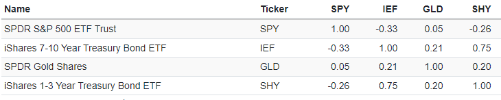
The correlations of these assets over the period 18 November 2004 - 11 August 2023 are displayed in Figure 1, adapted from Portfolio Visualizer.

Figure 1. SPY, IEF, GLD, SHY correlations over the period 18 November 2004 - 11 August 2023, based on daily returns. Source: Portfolio Visualizer.

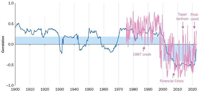
Before thinking about perturbing all these correlations, let’s assume that we would merely like to perturb the U.S. stock-bond correlation so as to bring it to a level representative of the pre-2000 period, like 0.5 or above, c.f. Figure 2 reproduced from Brixton et al.⁶.

Figure 2. Rolling Correlation between US Equity and US Treasury Returns, 01 January 1900 – 30 September 2022. Source: Brixton et al.

It turns out that this single perturbation already results in an invalid correlation matrix⁷!

As a consequence, trying to perturb the coefficients of a correlation matrix both simultaneously and at random has little chance to produce a valid correlation matrix in general, especially as the number of assets increases.

One solution to this issue is to replace the randomly perturbed correlation matrix by its nearest valid correlation matrix⁸, c.f. the post When a Correlation Matrix is not a Correlation Matrix: the Nearest Correlation Matrix Problem.

This leads to the following naive method to generate random perturbations of a correlation matrix $C \in \mathcal{M} \left( \mathbb{R}^{n \times n} \right)$:

1. Generate $\frac{n (n-1)}{2}$ randomly perturbed correlation coefficients $\widehat{C}_{i,j} \in [-1, 1]$ around the baseline correlation coefficients $C_{i,j}$, $i=1..n, j=i+1..n$
2. Compute the (potentially invalid) associated randomly perturbed correlation matrix $\widehat{C}$
3. Compute the randomly perturbed correlation matrix $\widetilde{C}$ as the nearest valid correlation matrix to $\widehat{C}$

While straightforward to implement⁹, this method has several limitations:

• It requires the computation of the nearest correlation matrix to every randomly perturbed correlation matrix generated

  Such systematic computation is expensive.

• It usually¹⁰ generates randomly perturbed correlation matrices that are singular

  This is because standard algorithms to compute the nearest correlation matrix, like Higham’s alternating projections algorithm⁸, output a singular correlation matrix¹¹.

• It provides no guarantee on the magnitude or on the distribution of the perturbations

  Due to the nearest correlation matrix step #3, it seems actually rather difficult to control either the magnitude or the probability distribution of the perturbations $ \left | C_{i,j} - \widehat{C}_{i,j} \right | $, $i=1..n$, $j=i+1..n$.

Hardin et al.’s method

Hardin et al.¹² introduce another method to randomly perturb the coefficients of a correlation matrix, relying on the dot product of normalized [independent gaussian random vectors]¹² as random perturbations.

One of the many advantages of this method compared to the naive method previously described is that the resulting randomly perturbed correlation matrix is a valid correlation matrix by construction, which allows to bypass the nearest correlation matrix step #3.

In details, given $C \in \mathcal{M} \left( \mathbb{R}^{n \times n} \right)$ a baseline correlation matrix, Hardin et al.’s method to generate random perturbations of $C$ works as follows:

1. Select a maximum noise level $\epsilon_{max}$ such that $0 < \epsilon_{max} < \lambda_{n}$, where $\lambda_{n}$ is the smallest eigenvalue of $C$

   $\epsilon_{max}$ controls the magnitude of the generated perturbations.

2. Select the dimension $m \geq 1$ of what is called the noise space in Hardin et al.¹²

   $m$ influences the distributional characteristics of the random perturbations, as depicted in Figure 3 adapted from Hardin et al.¹² on which it is visible that:

   • $m = 3$ produces uniform-like perturbations (S3)
   • $m = 25$ produces Gaussian-like perturbations (S25)

   

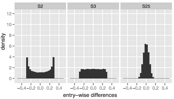
   Figure 3. Impact of the maximum noise level $\epsilon_{max}$ on the distribution of the perturbations (entry-wise differences). Source: Hardin et al.

3. Generate $n$ unit vectors $u_1,…,u_n$ belonging to $\mathbb{R}^{n}$ and construct the matrix $U \in \mathcal{M} \left( \mathbb{R}^{m \times n} \right)$ whose columns are the vectors $u_i, i=1..n$

4. Compute the randomly perturbed correlation matrix $\widetilde{C}$ as $\widetilde{C} = C + \epsilon_{max} \left( U{}^t U - I_n \right)$, where $I_n \in \mathcal{M} \left( \mathbb{R}^{n \times n} \right)$ is the identity matrix of order $n$

   The definition of $\widetilde{C}$ ensures that the perturbations are bounded by the maximum noise level $\epsilon_{max}$, i.e., $\left | C_{i,j} - \widetilde{C}_{i,j} \right | \leq \epsilon_{max} $, $i=1..n$, $j=i+1..n$.

Whenever possible, Hardin et al.’s method should be used (computationally cheap, possibility to control the perturbations in terms of magnitude and distribution…), although it suffers from two major limitations:

• It is not applicable to correlation matrices singular or close to singular

  This is due to the condition on the maximum noise level $\epsilon_{max}$ in step #1 and is regrettably a problem for applications in finance¹³, because as highlighted in Opdyke²:

  correlation matrices estimated on large portfolios often (perhaps usually) are not positive definite for a wide range of reasons, and once positive definiteness is enforced using reliable, proven methods […], the smallest eigenvalue of the resulting matrix is almost always virtually zero.

• It might not be applicable to a specific correlation matrix, even if not remotely close to singular

  This is again due to the condition on the maximum noise level $\epsilon_{max}$ in step #1.

  For instance, in the case of the Harry Browne’s permanent portfolio introduced in the previous sub-section, Hardin et al.’s method cannot be used to perturb the coefficients of the asset correlation matrix represented in Figure 1 by more than +/- 0.25¹⁴, and in particular, cannot be used to generate perturbed U.S. stock-bond correlations higher than -0.08¹⁵!

Random perturbations of the eigenvalues

The second family of methods to randomly perturb a correlation matrix is based on random perturbations of its eigenvalues.

A representative member of this family is the following method, with $C \in \mathcal{M} \left( \mathbb{R}^{n \times n} \right)$ a baseline correlation matrix to be perturbed:

1. Compute the eigendecomposition of $C$, with $C = P \Lambda P^{-1}$

2. Generate $n$ randomly perturbed eigenvalues $\widetilde{\lambda}_i \geq 0$ satisfying $\sum_{i=1}^n \widetilde{\lambda}_i = n$ around the baseline eigenvalues $\lambda_i$, $i=1..n$

   Galeeva et al.⁴ describe several algorithms and associated probability distributions that can be used in this step.

3. Compute the associated randomly perturbed diagonal matrix $\widetilde{\Lambda} = Diag \left( \widetilde{\lambda}_1,…, \widetilde{\lambda}_n \right)$
4. Compute the randomly perturbed correlation matrix $\widetilde{C}$ as $\widetilde{C} = P^{-1} \widetilde{\Lambda} P$

Any method from this family guarantees, in theory, the validity of the resulting randomly perturbed correlation matrix.

Nevertheless, in practice, Opdyke² notes that:

perturbing eigenvalues fails under challenging empirical conditions, e.g. when the positive definiteness of the matrix has to be enforced algorithmically […] and eigenvalues are virtually zero (or at least unreliably estimated)

In addition, controlling the $\frac{n (n-1)}{2}$ perturbations $\left | C_{i,j} - \widetilde{C}_{i,j} \right |$, $i=1..n$, $j=i+1..n$, which is ultimately what matters, through the $n$ perturbations $\left| \lambda_i - \widetilde{\lambda}_i \right|$, $i=1..n$, sounds rather difficult.

For these reasons, this family of methods might not be the first choice to generate random perturbations of a correlation matrix.

Random perturbations of the correlative angles

The third and last family of methods to randomly perturb a correlation matrix is based on random perturbations of its correlative angles.

Here, a representative member of this family is the following method, with $C \in \mathcal{M} \left( \mathbb{R}^{n \times n} \right)$ a baseline correlation matrix to be perturbed:

1. Compute the¹⁶ hypersphere decomposition of $C$, with $C = B B {}^t$
2. Generate $\frac{n (n-1)}{2}$ randomly perturbed correlative angles $\widetilde{\theta}_{i,j} \in [0, \pi]$ around the baseline correlative angles $\theta_{i,j}$, $i=1..n$, $j=1..i-1$
3. Compute the associated randomly perturbed lower triangular matrix $\widetilde{B}$
4. Compute the randomly perturbed correlation matrix $\widetilde{C}$ as $\widetilde{C} = \widetilde{B} \widetilde{B} {}^t$

Any method from this family again guarantees, in theory, the validity of the resulting randomly perturbed correlation matrix.

This time, though, theory seems to be confirmed in practice:

• Galeeva et al.⁴ highlight that perturbing the correlative angles is done via a robust and efficient procedure which makes the whole approach very attractive⁴
• Opdyke² notes that perturbing the correlative angles appears to be more robust [in practice] than competing methods […] at least under challenging empirical conditions²

One important remark at this stage is that the exact algorithms and associated probability distributions used in step #2 greatly influence the behavior of this family of methods.

For reference, Opdyke² proposes an algorithm called Cosecant, Cotangent, Cotangent (C3) able to generate a distribution of correlative angles median-centered on the baseline correlative angles and satisfying many other desirable properties¹⁷.

This algorithm generates a randomly perturbed correlative angle $\widetilde{\theta}_{i,j}$ around a baseline correlative angle $\theta_{i,j}$, $i=1..n$, $j=1..i-1$, as follows:

1. Generate a random variable $X$ of probability density function the p.d.f. of Makalic and Schmidt¹⁸ defined by $f_{X}(x) = c_k sin^k (x)$, $x \in (0, \pi)$, $k \geq 1$, where $c_k$ is a normalization constant and $k = n - j$
2. Compute the perturbed correlative angle $\widetilde{\theta}_{i,j}$ as $ \widetilde{\theta}_{i,j} = \arctan \left( \tan \left( \theta_{i,j}-\frac{\pi}{2} \right) + \tan \left( X - \frac{\pi}{2} \right) \right) + \frac{\pi}{2}$

This family of methods is particularly well-suited to what is called generalized (correlation) stress testing in Opdyke².

More on this later.

Still, like the family of methods based on random perturbations of the eigenvalues of a correlation matrix, one limitation of this family of methods is that controlling the $\frac{n (n-1)}{2}$ perturbations $\left | C_{i,j} - \widetilde{C}_{i,j} \right |$, $i=1..n$, $j=i+1..n$ sounds once again rather difficult.

Implementation in Portfolio Optimizer

Portfolio Optimizer allows to generate random perturbations of a baseline correlation matrix with:

• The naive method of randomly perturbing the coefficients of a correlation matrix

  Once a (potentially invalid) randomly perturbed correlation matrix is generated on client side, the endpoint /assets/correlation/matrix/nearest can be used to compute the nearest correlation matrix to this matrix.

• The method of randomly perturbing the correlative angles of a correlation matrix

  • Together with Opdyke’s C3 algorithm², through the endpoint /assets/correlation/matrix/perturbed

  • Together with a proprietary algorithm able to control the magnitude of the perturbations of the correlation coefficients, again through the endpoint /assets/correlation/matrix/perturbed

    In this case, the distribution of the randomly perturbed correlation matrices is asymptotically uniform over the space of positive definite correlation matrices whose distance in terms of max norm to the baseline correlation matrix is at most equal to (resp. exactly equal to) a given maximum noise level (resp. a given exact noise level), similar in spirit to the method of Hardin et al.¹²

Example of application - Generalized stress testing

Suppose that we are managing the Harry Browne’s permanent portfolio introduced earlier.

Suppose also that on 18 February 2020, we feel something is off and would like to assess the impact of a potential correlation breakdown on this portfolio.

Because this potential correlation breakdown could manifest in many ways (increased correlations between certain ETFs, decreased correlation between other ETFs…), it would be a mistake to impose any prior on how correlations should behave or should not behave¹⁹.

So, what could we do?

Direct correlation stress testing

Following the previous sections, one possibility is to generate random perturbations around the current correlation matrix of the ETFs in the portfolio, which will allow to simulate many potential correlation breakdowns in a prior-free way.

Once this is done, it will then be possible to evaluate the portfolio sensitivity to these random shocks.

Such a direct (correlation) stress testing procedure allows to catch difficult-to-anticipate and/or difficult-to quantify second and third order effects of a large, multivariate, impactful scenario (e.g. pandemic + economic upheaval)².

In order to apply this procedure to the portfolio at hand, three prerequisites are necessary:

• Estimating the current correlation matrix $C_{PP}$ of the ETFs in the portfolio

  I will estimate $C_{PP}$ as the correlation matrix of the four ETFs in the portfolio²⁰ over the 24-day period 14 January 2020 - 18 February 2020²¹, which gives

  \[C_{PP} \approx \begin{pmatrix} 1 & -0.81 & -0.82 & -0.65 & \\ -0.81 & 1 & 0.84 & 0.70 \\ -0.82 & 0.84 & 1 & 0.75 \\ -0.65 & 0.70 & 0.75 & 1 \end{pmatrix}\]

• Selecting a method to randomly perturb the current correlation matrix $C_{PP}$

  I will generate random perturbations of $C_{PP}$ thanks to Opdyke’s C3 algorithm² as implemented through the Portfolio Optimizer endpoint /assets/correlation/matrix/perturbed.

• Determining how to evaluate the portfolio sensitivity to the random perturbations of the current correlation matrix $C_{PP}$

  To keep things simple, I will evaluate the portfolio effective number of bets²² (ENB), using the Portfolio Optimizer endpoint /portfolio/analysis/effective-number-of-bets.

With these prerequisites met, it is possible to generate random perturbations around the current correlation matrix $C_{PP}$ and compute the corresponding ENB distribution.

An example of ENB distribution is provided in Figure 5, in the case of 10000 randomly perturbed correlation matrices.

Figure 5. Distribution of the Effective Number of Bets (ENB), 10000 randomly perturbed correlation matrices around the current correlation matrix $C_{PP}$.

Some associated summary statistics:

Mean	1.89
Standard deviation	0.42
Minimum	1.01
5% percentile	1.33
25% percentile	1.60
Median	1.81
75% percentile	2.12
95% percentile	2.72
Maximum	3.98

And, for reference, the value of the current ENB of the portfolio, computed with the current correlation matrix $C_{PP}$: 1.87.

A couple of comments:

• More than half of the ENB are located very close²³ to the current ENB (1.87)

  These ENB are not representative of any real correlation breakdown.

• The 95% percentile of the ENB distribution (2.72) is much further apart from the current ENB (1.87) than the 5% percentile of the ENB distribution (1.33)

  This means that a correlation breakdown with the biggest impact on the ENB would correspond, maybe counter-intuitively, to a scenario of de-correlation²⁴ of the four ETFs in the portfolio.

  As a side note, and again maybe counter-intuitively, the impact of such a correlation breakdown would then be rather harmless, because an increase in ENB is usually desirable from a portfolio diversification perspective.

• The minimum (1.01) and maximum (3.98) ENB both correspond to the theoretical minimum (1) and maximum (4) ENB

  This shows that all possible (correlation) unknown unknowns have been covered by the stress testing procedure.

Reverse correlation stress testing

In the previous sub-section, we have (empirically) established that the most impactful correlation breakdown scenario for the ENB of the portfolio corresponds to a de-correlation of the ETFs.

The next logical step is now to compute a correlation matrix that would somehow best illustrate this de-correlation scenario, a procedure known as reverse (correlation) stress testing.

For this, inspired by the concept of market states from Stepanov et al²⁵, I propose to apply a k-means clustering algorithm²⁶, with $k = 2$, to the randomly perturbed correlation matrices generated during the direct stress testing procedure.

One output of this algorithm is two “representative” correlation matrices²⁷, which are, in the case of the 10000 randomly perturbed correlation matrices of the previous sub-section:

• A correlation matrix $\widetilde{C}_{PP,1}$ “representative” of all the randomly perturbed correlation matrices that are “maximally similar” to the current correlation matrix $C_{PP}$

  \[\widetilde{C}_{PP,1} \approx \begin{pmatrix} 1 & -0.76 & -0.78 & -0.67 & \\ -0.76 & 1 & 0.75 & 0.66 \\ -0.78 & 0.75 & 1 & 0.67 \\ -0.67 & 0.66 & 0.67 & 1 \end{pmatrix}\]

• A correlation matrix $\widetilde{C}_{PP,2}$ “representative” of all the randomly perturbed correlation matrices that are “maximally dissimilar” from $\widetilde{C}_{PP,1}$

  \[\widetilde{C}_{PP,2} \approx \begin{pmatrix} 1 & -0.64 & -0.64 & -0.12 & \\ -0.64 & 1 & 0.53 & 0.07 \\ -0.64 & 0.53 & 1 & 0.06 \\ -0.12 & 0.07 & 0.06 & 1 \end{pmatrix}\]

, with “representative”, “maximally similar” and “maximally dissimilar” loosely defined but usually corresponding to intuition²⁸.

In terms of market states²⁵:

• The correlation matrix $\widetilde{C}_{PP,1}$ embodies the current market state

  Indeed, $\widetilde{C}_{PP,1}$ is very close to $C_{PP}$, as confirmed by the small Frobenius distance between these two matrices (0.21).

  In the current market state, the ENB is concentrated²⁹ around the current ENB of the portfolio (1.87).

• The correlation matrix $\widetilde{C}_{PP,2}$ embodies a market state maximally distinct from the current market state, which I will call the de-correlation market state

  The rationale for this name is that a comparison between $C_{PP}$ and $\widetilde{C}_{PP,2}$ shows that this second market state corresponds to a de-correlation of the four ETFs in the portfolio³⁰.

  In the de-correlation market state, the ENB is much higher that in the current market state, with for example the ENB computed with the correlation matrix $\widetilde{C}_{PP,2}$ equal to 2.97, well above the 95% percentile of the ENB distribution (2.72).

Thanks to these observations, it is possible to conclude that $\widetilde{C}_{PP,2}$ is the correlation matrix that best illustrate the most impactful correlation breakdown scenario for the ENB of the portfolio.

Reality check

I will conclude this example on generalized stress testing by a reality check on the results obtained in the previous sub-sections.

The correlation matrix $C_{PP, COVID}$ below is the correlation matrix of the four ETFs in the portfolio²⁰ over the subsequent 24-day “full crisis” period 19 February 2020 - 23 March 2020²¹.

\[C_{PP, COVID} \approx \begin{pmatrix} 1 & -0.50 & -0.40 & 0.00 & \\ -0.50 & 1 & 0.71 & 0.25 \\ -0.40 & 0.71 & 1 & 0.19 \\ 0.00 & 0.25 & 0.19 & 1 \end{pmatrix}\]

Of particular interest:

• The resemblance between $C_{PP, COVID}$ and $\widetilde{C}_{PP,2}$, confirmed by a relatively small Frobenius distance between these two matrices (0.58)
• The close match between the ENB computed with $C_{PP, COVID}$ (2.84) and the ENB computed with $\widetilde{C}_{PP,2}$ (2.97)

In other words:

• The most theoretically impactful correlation breakdown scenario for the ENB of the portfolio actually occurred in practice, with an associated asset correlation matrix relatively close to the forecast asset correlation matrix
• The forecast of the impact on the ENB of the portfolio of this theoretical correlation breakdown scenario was nearly spot on!

Conclusion

The possibility to generate random perturbations of a correlation matrix has many other applications in risk management and even beyond.

As an example, in mean-variance optimization, the resampled efficient frontier is partially based on random perturbations of a baseline correlation matrix.

Also, as a last remark on Opdyke’s C3 algorithm², a fully nonparametric version of it is described on Opdyke’s website.

This extended version, called Nonparametric Angles-based Correlation (NAbC), covers not only correlation matrices based on any underlying data distributions³¹ but also correlation matrices beyond the standard Pearson’s correlation matrix, like Spearman’s Rho correlation matrix or Kendall’s Tau correlation matrix.

For more random quantitative discussions, feel free to connect with me on LinkedIn or to follow me on Twitter.

–

1. Otherwise, these unknown unknows would become known unknows! ↩

2. See Opdyke, JD, Full Probabilistic Control for Direct and Robust, Generalized and Targeted Stressing of the Correlation Matrix (Even When Eigenvalues are Empirically Challenging) (May 30, 2020). QuantMinds/RiskMinds September 22-23, 2020. ↩ ↩² ↩³ ↩⁴ ↩⁵ ↩⁶ ↩⁷ ↩⁸ ↩⁹ ↩¹⁰ ↩¹¹ ↩¹²

3. See Rapisarda, F., Brigo, D. and Mercurio, F. (2007) Parameterizing correlations: a geometric interpretation, IMA Journal of Management Mathematics, 18(1), pp. 55–73. ↩

4. See Risk Management in Commodity Markets: From Shipping to Agriculturals and Energy, Chapter 6, Roza Galeeva, Jiri Hoogland, and Alexander Eydeland, Measuring Correlation Risk for Energy Derivatives. ↩ ↩² ↩³ ↩⁴

5. Of course, many other methods exist; for example, if the data generating process is known, it is possible to use a Monte-Carlo method to generate random samples from this process and compute their associated (sample) correlation matrix, which is then a perturbed version of the original correlation matrix. ↩

6. See A Changing Stock–Bond Correlation: Drivers and Implications, Alfie Brixton, Jordan Brooks, Pete Hecht, Antti Ilmanen, Thomas Maloney, Nicholas McQuinn, The Journal of Portfolio Management, Multi-Asset Special Issue 2023, 49 (4) 64 - 80. ↩

7. I’ll skip the math, but the interested reader can for example compute the eigenvalues of the asset correlation matrix represented in Figure 1 with the U.S. stock-bond correlation altered from -0.33 to 0.5. ↩

8. Nicholas J. Higham, Computing the Nearest Correlation Matrix—A Problem from Finance, IMA J. Numer. Anal. 22, 329–343, 2002. ↩ ↩²

9. Assuming that an algorithm to compute the nearest correlation matrix is available; otherwise, this method becomes immediately less straightforward to implement… ↩

10. Except if the initial randomly perturbed correlation matrices are actually valid, non-singular, correlation matrices. ↩

11. It is sometimes possible, though, to integrate an additional constraint on the minimum eigenvalue of the computed nearest valid correlation matrix into these algorithms. ↩

12. See Hardin, Johanna; Garcia, Stephan Ramon; Golan, David. A method for generating realistic correlation matrices. Ann. Appl. Stat. 7 (2013), no. 3, 1733–1762. ↩ ↩² ↩³ ↩⁴ ↩⁵

13. This is maybe less of a problem in other applications, like in biology. ↩

14. Because the smallest eigenvalue of the asset correlation matrix represented in Figure 1 is 0.25. ↩

15. Similarly, Hardin et al.’s method cannot be used to generate random pertubations of the U.S. stock-bond correlation that would bring this correlation to a level lower than -0.58. ↩

16. Strictly speaking, when the correlation matrix $C$ is positive semi-definite, its hypersphere decomposition is not unique. ↩

17. C.f. Opdyke² for the complete list of goals of his proposed approach. ↩

18. See Enes Makalic & Daniel F. Schmidt (2022) An efficient algorithm for sampling from sink(x) for generating random correlation matrices, Communications in Statistics - Simulation and Computation, 51:5, 2731-2735. ↩

19. For example, assuming that all correlations would go to one in case of a correlation breakdown is a prior. ↩

20. More specifically, of the daily arithmetic total returns of the four ETFs in the portfolio, whose prices have been retrieved using Tiingo. ↩ ↩²

21. I used a 24-day period because the period 19 February 2020 - 23 March 2020, which corresponds to the peak of the COVID financial crisis - c.f. Wikipedia - is also a 24-day period. ↩ ↩²

22. Due to personal preferences, I will use the effective number of bets based on principal components analysis as the factors extraction method; in addition, I will use the asset correlation matrix as if it were the asset covariance matrix to not introduce any additional variables (volatilities). ↩

23. More precisely, within a +/- 0.30 interval around 1.87. ↩

24. Intuitively, the higher the ENB of an equally-weighted portfolio, the more uncorrelated its constituents. ↩

25. See Stepanov, Y., Rinn, P., Guhr, T., Peinke, J., & Schafer, R. (2015). Stability and hierarchy of quasi-stationary states: financial markets as an example. Journal of Statistical Mechanics: Theory and Experiment, 2015(8), P08011. ↩ ↩²

26. I used the standard Scikit-Learn $k$-means algorithm. ↩

27. The k-means algorithm does not guarantee that the cluster centroids are valid correlation matrices; if this is not the case, it is possible to use either the $k$-medoids instead, or to compute the nearest correlation matrices to the cluster centroid. ↩

28. And more rigorously defined as per the $k$-means algorithm. ↩

29. To be noted that the ENB computed with the correlation matrix $C^{‘}_{PP,1}$ is nearly identical to the ENB computed with the current correlation matrix $C_{PP}$ (1.87). ↩

30. For example, U.S. stocks and Gold move from anti-correlated (-0.65) to nearly uncorrelated (-0.12). ↩

31. That is, data distributions characterized by any degree of serial correlation, asymmetry, non-stationarity, and/or heavy-tailedness. ↩