Managing Missing Asset Returns in Portfolio Analysis and Optimization: Backfilling through Residuals Recycling

In a multi-asset portfolio, it is usual that some assets have shorter return histories than others¹.

Problem is, the presence of assets whose return histories differ in length makes it nearly impossible to use standard portfolio analysis and optimization methods…

Estimating the historical covariance matrix of a multi-asset portfolio, for example, is not possible when assets have unequal return histories, so that a typical workaround used in practice is to consider only the common returns history. Unfortunately, this workaround has the side effect of discarding information contained in the longer return histories, which might greatly impact the quality of the estimated covariance matrix².

Sebastien Page proposes a solution to this problem in his paper How to Combine Long and Short Return Histories Efficiently³. It consists in simulating missing asset returns based on the relationships observed between all assets over their common returns history while accounting for the associated estimation error.

In this blog post, I will describe in detail Page’s method and analyze how it behaves empirically with a two-asset class portfolio made of U.S. and E.M. stocks.

Notes:

• A Jupyter notebook corresponding to this post is available on Binder -

Page’s method to backfill missing asset returns

Single starting date

Let be two groups of assets $X$ and $Y$ such that:

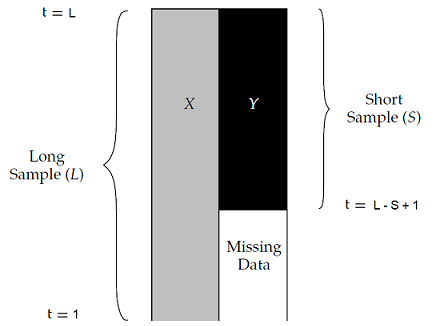
• The “long” group of assets $X = \left( X_1,…,X_n \right)$ is made of $n \geq 1$ assets, all sharing together a common returns history of length $L$
• The “short” group of assets $Y = \left( Y_1,…,X_m \right)$ is made of $m \geq 1$ assets, all sharing together a common returns history of length $S < L$ as well as sharing a common (ending) returns history of length $L - S + 1$ with the group of assets $X$

In such a situation, illustrated in Figure 1 adapted from Page³, returns for the group of assets $Y$ are missing for the whole (beginning) returns history $t = 1..L - S$.

Figure 1. Missing asset returns with a single starting date. Source: Page.

Building on the maximum likelihood procedure⁴ described in Stambaugh⁵, Page³ introduces a 3-step method in order to combine [these] long and short return histories efficiently³ and backfill the $ m \times \left( L - S \right)$ missing asset returns.

Step 1 - Estimation of the asset “long” mean returns

The vector $\hat{\mu}_{Y,L} \in \mathbb{R}^{m}$ of the mean returns of the assets belonging to the group $Y$ is estimated over the long returns history by:

\[\hat{\mu}_{Y,L} = \mu_{Y,S} + \beta \left( \mu_{X,L} - \mu_{X,S} \right)\]

, with:

• $\mu_{Y,S} = \left( \mu_{Y_1,S}, …, \mu_{Y_m,S} \right) {}^t \in \mathbb{R}^{m}$ the vector of the mean returns of the assets belonging to the group $Y$, computed over the short returns history
• $\beta \in \mathcal{M}(\mathbb{R}^{m \times n})$, the vector of standard regression coefficients defined by $\beta = \Sigma_{XX,S}^{-1} \Sigma_{XY,S}$, with:
  • $\Sigma_{XX,S} \in \mathcal{M}(\mathbb{R}^{n \times n})$ the covariance matrix of the assets belonging to the group $X$, computed over the short returns history
  • $\Sigma_{XY,S} \in \mathcal{M}(\mathbb{R}^{m \times n})$ the covariance matrix between the assets belonging to the group $X$ and the assets belonging to the group $Y$, computed over the short returns history
• $\mu_{X,L} = \left( \mu_{X_1,L}, …, \mu_{X_n,L} \right) {}^t \in \mathbb{R}^{n}$, the vector of the mean returns of the assets belonging to the group $X$, computed over the long returns history
• $\mu_{X,S} = \left( \mu_{X_1,S}, …, \mu_{X_n,S} \right) {}^t\in \mathbb{R}^{n}$, the vector of the mean returns of the assets belonging to the group $X$, computed over the short returns history

Step 2: Estimation of the asset long covariance matrix

The covariance matrix $\hat{\Sigma}_{YY,L} \in \mathcal{M}(\mathbb{R}^{m \times m})$ of the assets belonging to the group $Y$ is estimated over the long returns history by:

\[\hat{\Sigma}_{YY,L} = \Sigma_{YY,S} + \beta \left( \Sigma_{XX,L} - \Sigma_{XX,S} \right) \beta {}^t\]

, with:

• $\Sigma_{YY,S} \in \mathcal{M}(\mathbb{R}^{m \times m})$ the covariance matrix of the assets belonging to the group $Y$, computed over the short returns history
• $\Sigma_{XX,L} \in \mathcal{M}(\mathbb{R}^{n \times n})$ the covariance matrix of the assets belonging to the group $X$, computed over the long returns history

Similarly, the covariance matrix $\hat{\Sigma}_{XY,L} \in \mathcal{M}(\mathbb{R}^{m \times n})$ between the assets belonging to the group $X$ and the assets belonging to the group $Y$ is estimated over the long returns history by:

\[\hat{\Sigma}_{XY,L} = \Sigma_{XY,S} + \beta \left( \Sigma_{XX,L} - \Sigma_{XX,S} \right)\]

Step 3: Backfilling of the missing long asset returns

Once the long mean vectors and covariance matrix have been estimated thanks to step 1 and step 2, it is possible to simulate the missing (multivariate) asset returns $Y_t = \left( Y_{1,t},…,Y_{m,t} \right) {}^t \in \mathbb{R}^{m}$ for $t = 1..L - S$.

Page³ mentions 3 backfilling procedures for doing so, all based on a transformation of the long (multivariate) asset returns $X_t = \left( X_{1,t},…,X_{n,t} \right) {}^t \in \mathbb{R}^{n}$:

• Beta adjustment

  The beta adjustment backfilling procedure is based on the deterministic transformation:

  \[Y_t = \mu_{b_t}\]

  , with $\mu_{b_t} = \hat{\mu}_{Y,L} + \hat{\Sigma}_{XY,L} \Sigma_{XX,L}^{-1} \left( X_t - \mu_{X,L} \right) \in \mathbb{R}^{m}$

  The main problem with this procedure is that it gives a false sense of uniqueness for the backfilled asset returns.

  Indeed, as Page puts it³:

  […] the solution will not be unique: Many sets of simulated missing returns correspond to a given covariance matrix. This feature of the backfilling process is intuitive because, after all, the missing returns are unknown and so the model must recognize the uncertainty around the estimates.

  So, this backfilling procedure is probably best used only for bechmarking purposes.

• Conditional sampling

  In order to take into account estimation error into the backfilled asset returns, the conditional sampling backfilling procedure models the missing asset returns as a (multivariate) Gaussian distribution:

  \[Y_t \sim \mathcal{N} \left(\mu_{b_t}, \Sigma_b \right)\]

  , with:

  • $\mu_{b_t}$, defined in the beta adjustment backfilling procedure, the mean vector of the Gaussian distribution
  • $\Sigma_b = \hat{\Sigma}_{YY,L} - \hat{\Sigma}_{XY,L} \Sigma_{XX,L}^{-1} \hat{\Sigma}_{XY,L} {}^t \in \mathcal{M}(\mathbb{R}^{m \times m})$ the covariance matrix of the Gaussian distribution⁶

  Here, Page³ notes that at the null noise limit (i.e., $\Sigma_b = 0$), this backfilling procedure becomes equivalent to the beta adjustment backfilling procedure.

• Residuals recycling

  Modeling the missing asset returns by a Gaussian distribution might be appropriate in some cases, depending on the assets and on the returns measurement frequency⁷, but generally speaking, financial assets exhibit skewed and fat-tailed return distributions.

  So, it would make sense if backfilled asset returns were to take into account these characteristics.

  This is the aim of the residuals recycling backfilling procedure, which works as follows:

  • For $t = L - S + 1 .. T$, the difference $R_t$ between the (non-missing) asset returns $X_t$ and $\mu_{b_t}$, defined in the beta adjustment backfilling procedure, is computed
  \[R_t = X_t - \mu_{b_t}\]
  • For $t = 1..L - S$, the missing asset returns are backfilled as
  \[Y_t = \mu_{b_t} + R_{t'}\]

  , with $t’ \in [L - S + 1..T]$ chosen uniformly at random.

  Page³ highlights that this backfilling procedure represents a hybrid between [maximum likelihood estimation] and bootstrapping³ and that it provides a simple, relatively assumption-free approach to account for fat tails and other features of the distribution beyond means and covariances in the backfilling process.³.

Multiple starting dates

Page’s method as described in the previous paragraph assumes that all the assets belonging to the short group of assets $Y$ share a common returns history, and in particular a common returns history starting date.

In practice, though, most assets do not usually share a common returns history starting date, as illustrated in Figure 2 adapted from Gramacy et al.⁸.

Figure 2. Missing asset returns with several starting dates. Source: Gramacy et al.

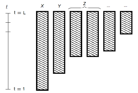
In such a situation, a possible way to extend Page’s method is to apply it iteratively as proposed in Jiang and Martin⁹.

For this, let be $G_1,…,G_J, J \geq 1$ groups of assets whose length of returns history $L = L_1 > L_2 > … > L_J \geq 1$ differ, but which share a common returns history ending date, as illustrated in Figure 2.

Then, Page’s method can be extended as follows:

• Apply Page’s method to the long group of assets $X = G_1$ and to the short group of assets $Y = G_2$
• Once missing asset returns in the group $Y = G_2$ have been backfilled, apply Page’s method to the long group of assets $X = G_1 \cup G_2$ and to the short group of assets $Y = G_3$
• …
• Once missing asset returns in the group $Y = G_{J-1}$ have been backfilled, apply Page’s method to the long group of assets $X = G_1 \cup G_2 \cup … \cup G_{J-1}$ and to the short group of assets $Y = G_J$

Practical details

Some numerical subtelties need to be taken into account when implementing Page’s method, among which that:

• The covariance matrix $\Sigma_{XX,S}$ of the assets belonging to the group $X$, computed over the short returns history, might not be invertible, c.f. for example Gramacy et al.⁸
• The covariance matrix $\Sigma_b$ of the Gaussian distribution appearing in the conditional sampling backfilling method might not be positive semi-definite

Caveats

Page³ highlights that his method does not magically transforms missing data into additional information³ and lists several of its limitations.

I think one of the most important of these is that³

The model assumes that betas between the existing [asset returns] and the missing [asset returns] do not change, which is not necessarily a realistic assumption.

To also be noted that even with this method, backfilling missing returns for a completely new asset class might unfortunately remain elusive.

For example, in their piece Risk Analysis of Crypto Assets, people at Two Sigma concludes that Bitcoin is not easily explained by the Two Sigma Factor Lens, nor is it substantially correlated to other currencies or any of the major commodities, so that no long returns history of any asset class seems to contain sufficient information to accurately backfill Bitcoin returns…

Implementation in Porfolio Optimizer

Portfolio Optimizer implements the extension of Page’s method for multiple starting dates described in the previous section, together with specific care for the numerical subtelties also described in the previous section, through the endpoint /assets/returns/backfilled.

Quality of backfilled returns

Page’s residuals recycling backfilling procedure has been designed to better account for non-normal distributions³.

To which extent is this goal reached in practice?

Let’s check.

Theoretical asset returns distribution

Page³ uses a simulation framework in order to compare backfilled v.s. expected returns for a bivariate $t$-distribution and obtain the results displayed in Figure 3, taken from Page³.

Figure 3. Higher moments for backfilled simulated returns compared with known bivariate fat-tailed t-distribution. Source: Page.

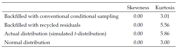
Results from Figure 3 leads to the following conclusions:

• Missing returns backfilled with the conditional sampling backfilling procedure converge to a (univariate) Gaussian distribution
• Missing returns backfilled with the residuals recycling backfilling procedure seem to have a sample kurtosis very close to the sample kurtosis of the theoretical bivariate $t$-distribution

In other words, the residuals recycling backfilling procedure seems to reach its advertised goal, at least when applied to a known theoretical distribution.

Empirical asset returns distribution

More empirically, Page³ uses monthly returns on:

• U.S. stocks, represented by the Wilshire 5000 Total Market Index
• E.M. stocks, represented by the MSCI Emerging Markets Index (Total Return)

in order to compare backfilled v.s. actual returns for E.M. stocks.

In more details:

• Returns on U.S. stocks from January 1988 to May 2011 (long returns history) and returns on E.M. stocks from February 1998 to May 2011 (short returns history) are used to backfill returns on E.M. stocks from January 1988 to January 1998¹⁰

  This process is repeated 10000 times to obtain 10000 different backfilled paths for emerging-market stocks³.

• Moments are computed on each backfilled path, and the grand average of these moments is computed over all backfilled paths

  The moments of interest are the mean, the variance, the skewness and the kurtosis of backfilled returns.

• Moments are computed on E.M. stocks using actual returns data from January 1988 to January 1998¹¹

Using Portfolio Optimizer, this test can easily be reproduced¹², c.f. the Jupyter notebook corresponding to this post, which gives for example the figures below:

Backfilling procedure	Mean	Variance	Skewness	Kurtosis
None (actual returns)	1.5%	0.0039	-0.25	3.83
Conditional sampling	2.2%	0.0036	-0.07	3.11
Recycled residuals	2.2%	0.0036	-0.20	3.24

These figures clearly show that the recycled residuals backfilling procedure generate asset returns that are closer, in terms of higher moments, to actual returns v.s. the conditional sampling backfilling procedure.

From this perspective, and even though the mean of backfilled returns is quite far off the mean of actual returns, the recycled residuals backfilling procedure can definitely be considered to properly recover fat tails in the missing [returns] data³.

Conclusion

Page’s method provides a formal, plug-and-play solution³ to the problem of unequal return histories in portfolio analysis and optimization.

While other methods certainly exist, like methods based on risk factors, these other methods usually tend to be more complex, so that Page’s method is a very good choice for anyone requiring a simple way to manage missing asset returns.

For more quantitative methods with just the right level of complexity, feel free to connect with me on LinkedIn or to follow me on Twitter.

–

1. For instance, historical returns of Emerging Markets (E.M.) stocks are available from the late 1980s¹³ while historical returns of U.S. stocks are available from the late 1920s¹⁴ or even earlier. ↩

2. See Steven P. Peterson, John T. Grier, Covariance Misspecification in Asset Allocation, Financial Analysts Journal, Vol. 62, No. 4 (Jul. - Aug., 2006), pp. 76-85. ↩

3. See Sebastien Page (2013) How to Combine Long and Short Return Histories Efficiently, Financial Analysts Journal, 69:1, 45-52. ↩ ↩² ↩³ ↩⁴ ↩⁵ ↩⁶ ↩⁷ ↩⁸ ↩⁹ ↩¹⁰ ↩¹¹ ↩¹² ↩¹³ ↩¹⁴ ↩¹⁵ ↩¹⁶ ↩¹⁷ ↩¹⁸ ↩¹⁹ ↩²⁰

4. Page³ note that in the context of his paper, asset returns series are not assumed to be multivariate Gaussian, so that the maximum likelihood procedure of Stambaugh actually becomes a quasi-maximum likelihood procedure. ↩

5. See Stambaugh, Robert F. 1997. Analyzing Investments Whose Histories Differ in Length. Journal of Financial Economics, vol. 45, no. 3 (September):285–331.. ↩

6. To be noted that contrary to $\mu_{b_t}$ , $\Sigma_b$ is time-independant. ↩

7. Asset returns have a tendency to follow a distribution closer and closer to a Gaussian distribution the more the time period over which they are computed increases; this empirical property is called aggregational Gaussianity, c.f. Cont¹⁵. ↩

8. See Robert B. Gramacy, Joo Hee Lee, Ricardo Silva, On estimating covariances between many assets with histories of highly variable length, arXiv. ↩ ↩²

9. See Jiang, Yindeng and Martin, R. Douglas, Turning Long and Short Return Histories into Equal Histories: A Better Way to Backfill Returns (August 31, 2016). ↩

10. To be noted that there is a typo in the heading of Table 3 in Page³, because known data is taken over January 1988 - January 1999, which is not 10 years but 20 years! ↩

11. Returns on E.M. stocks are indeed available from the full period January 1988 to May 2011. ↩

12. Results are not strictly identical to those of Page³, due to the random nature of the test; in addition, the skewness of actual E.M. returns is -0.26 in Page³ v.s. -0.25 here, probably due to some slight different in returns data. ↩

13. C.f. the MSCI website. ↩

14. C.f. the Kenneth French’s website. ↩

15. See R. Cont (2001) Empirical properties of asset returns: stylized facts and statistical issues, Quantitative Finance, 1:2, 223-236. ↩