Range-Based Volatility Estimators: Overview and Examples of Usage
Volatility estimation and forecasting plays a crucial role in many areas of finance.
For example, standard risk-based portfolio allocation methods (minimum variance, equal risk contributions, hierarchical risk parity…) critically depend on the ability to build accurate volatility forecasts1.
Multiple methods for estimating volatility have been proposed over the past several decades, and in this blog post I will focus on range-based volatility estimators.
These estimators, the first of which introduced by Parkinson2 as a way to compute the true variance of the rate of return of a common stock2, rely on the highest and lowest prices of an asset over a given time period to estimate its volatility, hence their name3.
After describing the four most well known range-based volatility estimators, I will reproduce the analysis of Arthur Sepp in his presentation Volatility Modelling and Trading4 made at Global Derivatives Conference 2016 and test the predictive power of the naive volatility forecasts produced by these estimators for various ETFs.
Notes:
A very accessible series of papers about range-based volatility estimators has recently5 been released by people at Lombard Odier, c.f. here, here and here.
Mathematical preliminaries
Volatility modelling
One of the main6 assumptions made when working with range-based volatility estimators7 is that the price movements $S_t$ of the asset under consideration follow a geometric Brownian motion with unknown volatility coefficient8 $\sigma$ and unknown drift coefficient $\mu$, that is
\[d S_t = \mu S_t dt + \sigma S_t dW_t\], where $W_t$ is a standard Brownian motion.
Under this working assumption, $\sigma$ represents the volatility of the asset.
Volatility and variance estimators
Although anyone can empirically observe the impact of “volatility” on the prices of a given asset, the volatility coefficient $\sigma$ of this asset is not directly observable9 and must be estimated using stock market information.
A statistical estimator of $\sigma$ is then called a volatility estimator, and a statistical estimator of $\sigma^2$ is called a variance estimator.
Efficiency of a volatility estimator
In order to determine the quality of a volatility estimator, two measures are commonly used:
-
The bias of a volatility estimator measures whether this estimator produces, on average, too high or too low volatility estimates.
More formally, a volatility estimator $\sigma_A$ is said to be unbiased when $\mathbb{E}[\sigma_A] = \sigma$ and biased otherwise.
-
The efficiency of a volatility estimator measures the uncertainty of the volatility estimates produced by this estimator, with the greater the efficiency of the estimator, the more accurate the volatility estimates.
More formally, the relative efficiency $Eff \left( \sigma_A \right)$ of a volatility estimator $\sigma_A$ compared to a reference volatility estimator $\sigma_B$ is defined as the ratio of the variance of the estimator $\sigma_B^2$ over the variance of the estimator $\sigma_A^2$, that is,
\[Eff \left( \sigma_A \right) = \frac{Var \left( \sigma_B^2 \right)}{Var \left( \sigma_A^2 \right)}\]
To be noted that bias and efficiency are sometimes conflicting, which is more generally known in statistics as the bias-variance tradeoff.
Close-to-close volatility estimators
Let $C_1,…,C_T$ be the closing prices of an asset for $T$ time periods $t=1..T$10.
Then,
\[\sigma_{cc,0} \left( T \right) = \sqrt{ \frac{1}{T-1} \sum_{i=2}^T \ln{\frac{C_i}{C_{i-1}}}^2 }\]is a biased11 estimator of the asset volatility $\sigma$ over the $T$ time periods, assuming zero drift (i.e., $\mu = 0$), c.f. Parkinson2.
In addition,
\[\sigma_{cc} \left( T \right) = \sqrt{ \frac{1}{T-2} \sum_{i=2}^T \left( \ln \frac{C_i}{C_{i-1}} - \mu_{cc} \right)^2 }\], with $\mu_{cc} = \frac{1}{T-1} \sum_{i=2}^T \ln \frac{C_i}{C_{i-1}} $, is a biased11 estimator of the asset volatility $\sigma$ over the $T$ time periods, assuming non-zero drift (i.e., $\mu \ne 0$), c.f. Yang and Zhang12.
These two estimators are known as close-to-close volatility estimators.
Range-based volatility estimators
Let be:
- $t=1..T$, $T$ time periods10
- $\left( O_1,H_1,L_1,C_1 \right), …, \left( O_T,H_T,L_T,C_T \right)$, the opening, highest, lowest and closing prices of an asset for time periods $t=1..T$
As mentioned in the introduction, a volatility estimator fully or partially relying on the highest prices $H_t, t=1..T$ and on the lowest prices $L_t, t=1..T$ is called a range-based volatility estimator.
The underlying idea behind such estimators is that information contained in the asset high-low price ranges $H_t - L_t, t=1..T$ should allow to build volatility estimators that are more efficient than the close-to-close volatility estimators, which use only one price inside this range13.
This quest for efficiency is important because, contrary to one of the working assumptions6, the volatility of an asset is known to be time-varying14, so that the less the number of time periods required to estimate its volatility, the more chances that its volatility is constant(ish) over the time periods under consideration.
As Rogers et al.15 put it:
[…] volatility may change over long periods of time; a highly efficient procedure will allow researchers to estimate volatility with a small number of observations.
Parkinson volatility estimator
Parkinson2 introduces an estimator for the diffusion coefficient of a Brownian motion without drift that relies on the highest and lowest observed values of this Brownian motion over a given time period.
When applied to the estimation of an asset volatility, this gives the Parkinson volatility estimator $\sigma_{P} \left( T \right)$ defined over $T$ time periods by
\[\sigma_{P} \left( T \right) = \sqrt{\frac{1}{T}} \sqrt{\frac{1}{4 \ln 2} \sum_{i=1}^T \left( \ln \frac{H_i}{L_i} \right) ^2}\]Intuitively, the Parkinson estimator should be “better” than the close-to-close estimators because large price movements impacting the high-low price range $H_t - L_t$ but leaving the closing price $C_t$ unchanged might occur within any time period $t$.
This is confirmed by the efficiency of this estimator, up to 5.2 times higher than the efficiency of the close-to-close estimators16.
Garman-Klass volatility estimator
Garman and Klass17 propose to improve the Parkinson estimator by taking into account the opening prices $O_t, t=1..T$ and the closing prices $C_t, t=1..T$.
This leads to the Garman-Klass volatility estimator $\sigma_{GK} \left( T \right)$, defined over $T$ time periods by
\[\sigma_{GK} \left( T \right) = \sqrt{\frac{1}{T}} \sqrt{ \sum_{i=1}^T \frac{1}{2} \left( \ln\frac{H_i}{L_i} \right) ^2 - \left( 2 \ln2 - 1 \right) \left( \ln\frac{C_i}{O_i} \right )^2 }\]For the historical comment, Garman and Klass17 establish in their paper that $\sigma_{GK}$ is the “best reasonable”18 volatility estimator that depends only on the high-open price range $H_t - O_t$, the low-open price range $L_t - O_t$ and the close-open price range $C_t - O_t$, $t=1..T$.
The Garman-Klass estimator is up to 7.4 times more efficient than the close-to-close estimators16.
Rogers-Satchell volatility estimator
The Parkinson and the Garman-Klass estimators have both been derived under a zero drift assumption.
When this assumption is not verified for an asset, for example because of a strong upward or downward trend in the asset prices or because of the usage of large time periods (monthly, yearly…), these estimators should in theory not be used because the quality of their volatility estimates is negatively impacted by the presence of a non-zero drift1915.
In order to solve this problem, Rogers and Satchell19 devise the Rogers-Satchell volatility estimator $\sigma_{RS} \left( T \right)$, defined over $T$ time periods by
\[\sigma_{RS} \left( T \right) = \sqrt{\frac{1}{T}} \sqrt{ \sum_{i=1}^T \ln\frac{H_i}{C_i} \ln\frac{H_i}{O_i} + \ln\frac{L_i}{C_i} \ln\frac{L_i}{O_i} }\]The Rogers-Satchell estimator is up to 6 times more efficient than the close-to-close estimators19, which is less than the Garman-Klass estimator20.
Yang-Zhang volatility estimator
The range-based volatility estimators discussed so far do not take into account opening jumps in an asset prices21, that is, the potential difference between an asset opening price $O_t$ and its closing price $C_{t-1}$ for a time period $t$22.
This limitation causes a systematic underestimation of the true volatility12.
When trying to integrate opening jumps into the Parkinson, the Garman-Klass and the Rogers-Satchell estimators, Yang and Zhang12 discover that it is unfortunately not possible for any “reasonable” single-period23 volatility estimator to properly handle both a non-zero drift and opening jumps.
This leads them to introduce the multi-period23 Yang-Zhang volatility estimator $\sigma_{YZ} \left( T \right)$, defined over $T$ time periods by
\[\sigma_{YZ} \left( T \right) = \sqrt{ \sigma_{ov}^2+ k \sigma_{oc}^2 + (1-k ) \sigma_{RS}^2 ) }\], where:
-
$\sigma_{co} \left( T \right)$ is the close-to-open volatility, defined as
\[\sigma_{co} = \sqrt{\frac{1}{T-2} \sum_{i=2}^T \left( \ln \frac{O_i}{C_{i-1}} - \mu_{co} \right)^2}\], with $\mu_{co} = \frac{1}{T-1} \sum_{i=2}^T \ln \frac{O_i}{C_{i-1}}$
-
$\sigma_{oc} $ is the open-to-close volatility, defined as
\[\sigma_{oc} \left( T \right) = \sqrt{\frac{1}{T-2} \sum_{i=2}^T \left( \ln \frac{O_i}{C_{i}} - \mu_{oc} \right)^2}\], with $\mu_{oc} = \frac{1}{T-1} \sum_{i=2}^T \ln \frac{C_i}{O_{i}}$
-
$\sigma_{RS}$ is the Rogers-Satchell volatility estimator over the time periods $t=2..T$
-
$k = \frac{0.34}{1.34 + \frac{T}{T-2}}$
In addition to the new estimator $\sigma_{YZ}$, Yang and Zhang12 also provide multi-period versions of the Parkinson, the Garman-Klass and the Rogers-Satchell estimators that support opening jumps24.
The Yang-Zhang estimator is up to 14 times more efficient than the close-to-close estimators12, a result that Yang and Zhang12 comment as follows
The improvement of accuracy over the classical close-to-close estimator is dramatic for real-life time series
Other estimators
The family of range-based volatility estimators has many other members:
- The Kunitomo25 volatility estimator
- The Alizadeh-Brandt-Diebold26 volatility estimator
- The Meilijson27 volatility estimator
- …
Still, the Parkinson, the Garman-Klass, the Rogers-Satchell and the Yang-Zhang volatility estimators are representative of this family, so that I will not detail any other range-based volatility estimator in this blog post.
From volatility estimation to volatility forecasting
Range-based volatility estimators are based on the assumption of independent sample and observations within the sample4, so that the corresponding volatility forecasts are simply naive forecasts under a random walk model.
In other words, with such volatility estimators, the “natural” forecast of an asset volatility over the next $T$ time periods is the (past) estimate of the asset volatility over the last $T$ time periods.
That being said, it is perfectly possible to use range-based volatility estimates together with any volatility forecasting model such as:
- A time series forecasting model like a simple or an exponentially weighted moving average model, as detailed for example in Jacob and Vipul28
- An econometric forecasting model like the GARCH model, c.f. Mapa29
- A specific range-based forecasting model (Chou’s30 Conditional AutoRegressive Range model, Harris and Yilmaz’s31 hybrid multivariate exponentially weighted moving average model…)
Performance of range-based volatility estimators
Theoretical and practical performances of range-based volatility estimators are studied in several papers, for example Shu and Zhang32, Jacob and Vipul28 and Brandt and Kinlay33, among others.
Most of these studies agree that range-based volatility estimators are biased11, but other conclusions differ depending on the exact methodology used.
In particular, as highlighted by Brandt and Kinlay33, the results from empirical research differ significantly from those seen in simulation studies in a number of respects33.
One perfect example of these differences is Shu and Zhang32 concluding, using a Monte Carlo simulation, that
If the drift term is large, the Parkinson estimator and the [Garman-Klass] estimator will significantly overestimate the true variance […]
, while Jacob and Vipul28 concluding, using real stock market data, that
Overall, the [Garman-Klass] estimator, which indirectly adjusts for the drift, performs better for the high-drift stocks.
Motivated by such inconsistencies, Lyocsa et al.34, building on Patton and Sheppard35, introduced what I will call the Lyocsa-Plihal-Vyrost volatility estimator $\sigma_{LPV}$, defined as the arithmetic average of the Parkinson, the Garman-Klass and the Rogers-Satchell volatility estimators36
\[\sigma_{LPV} = \frac{\sigma_{P} + \sigma_{GK} + \sigma_{RS}}{3}\]As Lyocsa et al.34 explain, the motivation behind using the (naive) equally weighted average is based on the assumption that we have no prior information on which estimator might be more accurate34.
I personally like the idea of an averaged estimator, but at this point, I think it is safe to highlight that there is no “best” range-based volatility estimator…
Implementation in Portfolio Optimizer
Portfolio Optimizer implements all the volatility estimators discussed in this blog post:
- The close-to-close volatility estimators, through the endpoint
/assets/volatility/estimation/close-to-close - The Parkinson volatility estimator, through the endpoint
/assets/volatility/estimation/parkinson - The Garman-Klass volatility estimator, through the endpoint
/assets/volatility/estimation/garman-klass - The original Garman-Klass volatility estimator18, through the endpoint
/assets/volatility/estimation/garman-klass/original - The Rogers-Satchell volatility estimator, through the endpoint
/assets/volatility/estimation/rogers-satchell - The Yang-Zhang volatility estimator, through the endpoint
/assets/volatility/estimation/yang-zhang
, as well as their jump-adjusted variations, whenever applicable.
Examples of usage
To illustrate possible uses of range-based volatility estimators, I propose to reproduce a couple of results from Sepp4:
- The estimation and the forecast of the SPY ETF monthly volatility
- The forecast of the monthly volatility of misc. ETFs representative of different asset classes (U.S. treasuries, international stock market, gold…)
Such examples will allow to compare the empirical behavior of the different volatility estimators and maybe reach a conclusion as to their relative performance in this specific setting.
Estimating SPY ETF volatility
I will estimate the SPY ETF monthly volatility using all the daily open/high/low/close prices37 observed during that month38.
Figure 1, limited to 5 volatility estimators for readability purposes, illustrates the results obtained over the period 31 January 2005 - 29 February 201639.
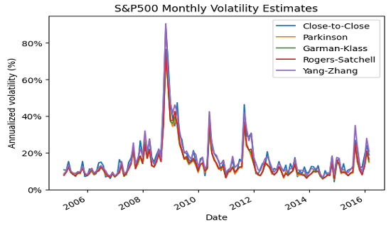
Figure 1 is mostly identical to the figure on slide 22 from Sepp4, on which it seems in particular that the close-to-close and the Yang-Zhang volatility estimators provide higher estimates of volatility when the overall level of volatility is high4.
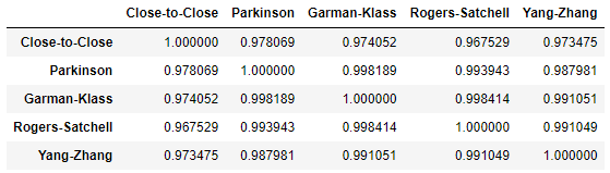
Overall, though, the behavior of the different volatility estimators is essentially the same on this specific example, which is confirmed by their correlations displayed in Figure 2.
Forecasting misc. ETFs volatility
Using the same methodology as in Sepp4, I will now evaluate the quality of the naive forecasts produced by all the range-based volatility estimators implemented in Portfolio Optimizer against the next month’s close-to-close observed volatility40, for 10 ETFs representative of misc. asset classes:
- U.S. stocks (SPY ETF)
- European stocks (EZU ETF)
- Japanese stocks (EWJ ETF)
- Emerging markets stocks (EEM ETF)
- U.S. REITs (VNQ ETF)
- International REITs (RWX ETF)
- U.S. 7-10 year Treasuries (IEF ETF)
- U.S. 20+ year Treasuries (TLT ETF)
- Commodities (DBC ETF)
- Gold (GLD ETF)
These ETFs are used in the Adaptative Asset Allocation strategy from ReSolve Asset Management, described in the paper Adaptive Asset Allocation: A Primer41.
For each ETF, Sepps’s methodology is as follows:
-
At each month’s end, compute the volatility estimates $\sigma_{cc, t}$, $\sigma_{P, t}$, … using all the ETF daily open/high/low/close prices37 observed during that month38
Under a random walk volatility model, each of these estimates represents the next month’s volatility forecast $\hat{\sigma}_{t+1}$
-
At each month’s end, also compute the next month’s close-to-close volatility estimate $\sigma_{cc, t+1}$ using all the ETF daily close prices37 observed during that month38
This estimate is the volatility benchmark, which represents how the ETF “volatility” is perceived by an investor monitoring her portfolio daily.
-
Once all months have been processed that way, regress the volatility forecasts on the volatility benchmarks by applying the Mincer-Zarnowitz42 regression model:
\[\hat{\sigma}_{t+1} = \alpha + \beta \sigma_{cc, t+1} + \epsilon_{t+1}\], where $\epsilon_{t+1}$ is an error term.
Then, the estimator producing [the best] volatility forecast is indicated by [a] high explanatory power R^2, [a] small intercept $\alpha$ and [a] $\beta$ coefficient close to one4.
Forecasting SPY ETF volatility
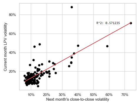
In the case of the SPY ETF, Figure 3 illustrates Sepps’s methodology for the Lyocsa-Plihal-Vyrost volatility estimator $\sigma_{LPV}$ over the period 31 January 2005 - 29 February 2016.
Detailed results for all regression models over the period 31 January 2005 - 29 February 2016:
| Volatility estimator | $\alpha$ | $\beta$ | $R^2$ |
|---|---|---|---|
| Close-to-close | 4.1% | 0.75 | 57% |
| Close-to-close (zero drift) | 3.9% | 0.77 | 57% |
| Parkinson | 3.5% | 0.95 | 58% |
| Parkinson (jump-adjusted) | 3.4% | 0.79 | 58% |
| Garman-Klass | 3.7% | 0.92 | 57% |
| Garman-Klass (jump-adjusted) | 3.6% | 0.77 | 58% |
| Garman-Klass (original) | 3.7% | 0.92 | 57% |
| Garman-Klass (original, jump-adjusted) | 3.6% | 0.77 | 58% |
| Rogers-Satchell | 4.0% | 0.88 | 56% |
| Rogers-Satchell (jump-adjusted) | 3.9% | 0.74 | 57% |
| Yang-Zhang | 3.8% | 0.75 | 58% |
| Lyocsa-Plihal-Vyrost | 3.7% | 0.92 | 57% |
While these figures are far43 from those on slide 42 from Sepp4, with for example nearly no variation in terms of $R^2$ among the different volatility estimators, two observations are similar:
- All volatility estimators have comparable $\alpha$
- The Parkinson, the Garman-Klass and the Rogers-Satchell volatility estimators have a $\beta$ much closer to 1 than the close-to-close volatility estimator
Forecasting the other ETFs volatility
Going beyond the SPY ETF, averaged results for all ETFs/regression models over each ETF price history44 are the following:
| Volatility estimator | $\bar{\alpha}$ | $\bar{\beta}$ | $\bar{R^2}$ |
|---|---|---|---|
| Close-to-close | 5.8% | 0.66 | 44% |
| Close-to-close (zero drift) | 5.6% | 0.67 | 45% |
| Parkinson | 5.6% | 0.94 | 44% |
| Parkinson (jump-adjusted) | 4.9% | 0.70 | 45% |
| Garman-Klass | 5.7% | 0.93 | 43% |
| Garman-Klass (jump-adjusted) | 5.0% | 0.70 | 44% |
| Garman-Klass (original) | 5.7% | 0.93 | 43% |
| Garman-Klass (original, jump-adjusted) | 5.0% | 0.70 | 44% |
| Rogers-Satchell | 6.1% | 0.88 | 42% |
| Rogers-Satchell (jump-adjusted) | 5.2% | 0.68 | 43% |
| Yang-Zhang | 5.1% | 0.69 | 44% |
| Lyocsa-Plihal-Vyrost | 5.7% | 0.92 | 43% |
A couple of remarks:
- Forecasts produced by all the volatility estimators explain on average only ~45% of the variability of the ETFs monthly volatility
- Forecasts produced by the jump-adjusted volatility estimators seem to offer no improvement on average over the forecasts produced by the close-to-close volatility estimator
- Forecasts produced by the Parkinson, the Garman-Klass and the Rogers-Satchell volatility estimators seem to be much less biased on average than the forecasts produced by the close-to-close volatility estimator, a property inherited by the Lyocsa-Plihal-Vyrost volatility estimator
As an empirical conclusion, it is disappointing that the naive monthly volatility forecasts produced by range-based volatility estimators have about the same predictive power as the forecasts produced by the close-to-close volatility estimator. Nevertheless, because these forecasts are much less biased than their close-to-close counterparts, they still represent an improvement for the many investors who currently rely on close prices only45.
To also be noted, similar to one of the conclusions of Lyocsa et al.34, that the Lyocsa-Plihal-Vyrost volatility estimator should probably be preferred to the Parkinson, the Garman-Klass or the Rogers-Satchell volatility estimators because using only one range-based estimators has occasionally led to very inaccurate forecasts, which could successfully be avoided by using the average of the three range-based estimators34.
Conclusion
One aspect of range-based volatility estimators not discussed in this blog post is their capability to capture important stylized facts about asset returns46.
This, together with possible ways to incorporate them in more predictive volatility models than the random walk model, will be the subject of future blog posts.
Meanwhile, for more volatile discussions, feel free to connect with me on LinkedIn or to follow me on Twitter.
–
-
As well as correlation forecasts. ↩
-
See Parkinson, Michael H., The Extreme Value Method for Estimating the Variance of the Rate of Return, The Journal of Business 53 (1980), 61-65, which is the final version of the working paper The random walk problem: extreme value method for estimating the variance of the displacement (diffusion constant) started 4 years before. ↩ ↩2 ↩3 ↩4
-
Because the range of prices of an asset over a given time period is contained, by definition, within its highest and its lowest price. ↩
-
See Sepp, Artur, Volatility Modelling and Trading. Global Derivatives Workshop Global Derivatives Trading & Risk Management, Budapest, 2016. ↩ ↩2 ↩3 ↩4 ↩5 ↩6 ↩7 ↩8
-
At the date of publication of this post. ↩
-
Other working assumptions are also commonly made, like assuming that the asset does not pay dividends, assuming that the volatility coefficient $\sigma$ remains constant, assuming that the geometric Brownian motion model also applies during time periods with no trading activity (e.g., stock market closure), etc. ↩ ↩2
-
In details, the geometric Brownian motion assumption slightly differs between authors; for example, Garman and Klass17 assume that asset prices follow a more generic diffusion process, which includes the geometric Brownian motion as a specific case. ↩
-
$\sigma$ is also called the diffusion coefficient of the geometric Brownian motion, but in the context of this blog post, I think it is clearer to explicitly call it the volatility coefficient. ↩
-
See Andersen, T., Bollerslev, T., Diebold, F., & Labys, P. (2003). Modeling and forecasting realized volatility. Econometrica, 71, 579–625. ↩
-
In practice, a time period $t$ usually corresponds to a trading day, a week or a month, so that the closing prices $C_t, t=1..T$ are simply the daily, weekly or monthly closing prices of the asset. ↩ ↩2
-
These estimators are biased, due to Jensen’s inequality; c.f. also Molnar46. ↩ ↩2 ↩3
-
See Yang, D., and Q. Zhang, 2000, Drift-Independent Volatility Estimation Based on High, Low, Open, and Close Prices, Journal of Business 73:477–491. ↩ ↩2 ↩3 ↩4 ↩5 ↩6
-
The asset closing price $C_t, t=1..T$. ↩
-
See French, K. R., Schwert, G. W., & Stambaugh, R. F. (1987). Expected stock returns and volatility. Journal of Financial Economics, 19, 3–29. ↩
-
See L. C. G. Rogers, S. E. Satchell & Y. Yoon (1994) Estimating the volatility of stock prices: a comparison of methods that use high and low prices, Applied Financial Economics, 4:3, 241-247. ↩ ↩2
-
See Colin Bennett, Trading Volatility, Correlation, Term Structure and Skew. ↩ ↩2
-
See Garman, M. B., and M. J. Klass, 1980, On the Estimation of Security Price Volatilities from Historical Data, Journal of Business 53:67–78. ↩ ↩2 ↩3
-
More precisely, Garman and Klass17 establish that a variation of $\sigma_{GK}$ is the “best” reasonable estimator but note that $\sigma_{GK}$ is 1) more practical and 2) as efficient as this variation, which I will call the original Garman-Klass volatility estimator $\sigma_{GKo}$. ↩ ↩2
-
See L. C. G. Rogers and S. E. Satchell, Estimating Variance From High, Low and Closing Prices, The Annals of Applied Probability, Vol. 1, No. 4 (Nov., 1991), pp. 504-512. ↩ ↩2 ↩3
-
Such a decrease in efficiency cannot be avoided because the Rogers-Satchell estimator belongs to class of estimators studied in Garman and Klass17, so that its efficiency is necessarily smaller than the efficiency of the Garman-Klass estimator (maximal by definition). ↩
-
Garman and Klass17 provide a volatility estimator that takes into account opening jumps, but this estimator has a dependency on an unknown $f$ parameter which makes it unusable in practice; Yang and Zhang12 show that this dependency is actually spurious and provide a usable form of this estimator. ↩
-
When the time periods $t$ are measured in trading days, opening jumps are called overnight jumps. ↩
-
A single-period volatility estimator is a volatility estimator that can be used to estimate the volatility of an asset over a single time period $t$ using price data for this time period only; for example, the Parkinson, the Garman-Klass and the Rogers-Satchell estimators are single-period estimators while the close-to-close estimators are multi-period estimators. ↩ ↩2
-
See Kunitomo, N. (1992). Improving the Parkinson method of estimating security price volatilities. Journal of Business, 65, 295–302. ↩
-
See Alizadeh ,S., Brandt, W. M., and Diebold, X.F., 2002. Range-based estimation of stochastic volatility models. Journal of Finance 57: 1047-1091. ↩
-
See Meilijson , I. (2011). The Garman–Klass Volatility Estimator Revisited. REVSTAT-Statistical Journal, 9(3), 199–212. ↩
-
See Jacob, J. and Vipul, (2008), Estimation and forecasting of stock volatility with range-based estimators. J. Fut. Mark., 28: 561-581. ↩ ↩2 ↩3
-
See Mapa, Dennis S., 2003. A Range-Based GARCH Model for Forecasting Volatility, MPRA Paper 21323, University Library of Munich, Germany. ↩
-
See Chou, R.Y. (2005). Forecasting Financial Volatilities with Extreme Values: The Conditional Autoregressive Range (CARR) Model. Journal of Money Credit and Banking, 37(3): 561-582. ↩
-
See Harris, R. D. F., & Yilmaz, F. (2010). Estimation of the conditional variance–covariance matrix of returns using the intraday range. International Journal of Forecasting, 26, 180–194. ↩
-
See Shu, J. and Zhang, J.E. (2006), Testing range estimators of historical volatility. J. Fut. Mark., 26: 297-313. ↩ ↩2
-
See Brandt, Michael W. and Kinlay, J, Estimating Historical Volatility (March 10, 2005). ↩ ↩2 ↩3
-
See Lyocsa S, Plihal T, Vyrost T. FX market volatility modelling: Can we use low-frequency data? Financ Res Lett. 2021 May;40:101776. doi: 10.1016/j.frl.2020.101776. Epub 2020 Sep 30. ↩ ↩2 ↩3 ↩4 ↩5
-
See Patton A.J., Sheppard K. Optimal combinations of realised volatility estimators. Int. J. Forecast. 2009;25(2):218–238. ↩
-
The Yang-Zhang volatility estimator is excluded to avoid mixing jump-adjusted volatility estimators with non-jump-adjusted ones. ↩
-
(Adjusted) prices have have been retrieved using Tiingo. ↩ ↩2 ↩3
-
The jump-adjusted Yang-Zhang volatility estimator, as well as the close-to-close volatility estimators, require the closing price of the last day of the previous month as an additional price. ↩ ↩2 ↩3
-
This period more or less matches with the period used in Sepp4. ↩
-
The next month’s close-to-close volatility is then taken as a proxy for the next month’s realized volatility; this choice is important, because different proxies might result in different conclusions as to the out-of-sample forecast performances. ↩
-
See Butler, Adam and Philbrick, Mike and Gordillo, Rodrigo and Varadi, David, Adaptive Asset Allocation: A Primer. ↩
-
See Mincer, J. and V. Zarnowitz (1969). The evaluation of economic forecasts. In J. Mincer (Ed.), Economic Forecasts and Expectations. ↩
-
This is due to slight differences in methodology, with mainly 1) the definition of “monthly volatility” in Sepp4 taken to be the volatility from the 3rd Friday of a month to the 3rd Friday of the next month and 2) the usage in Sepp4 of a linear regression model robust to outliers. ↩
-
The common ending price history of all the ETFs is 31 August 2023, but there is no common starting price history, as all ETFs started trading on different dates. ↩
-
For example, for all investors running some kind of monthly tactical asset allocation strategy. ↩
-
See Peter Molnar, Properties of range-based volatility estimators, International Review of Financial Analysis, Volume 23, 2012, Pages 20-29,. ↩ ↩2 ↩3