Correlation Matrix Stress Testing: Shrinkage Toward the Lower and Upper Bounds of a Correlation Matrix

I previously described on this blog an intuitive way of performing stress tests on a correlation matrix, which consists in shrinking a baseline correlation matrix toward an equicorrelation matrix¹².

A limitation of this method, though, is that it alters all the correlation coefficients of the baseline correlation matrix, so that it is for example impossible to stress only the correlation between two assets - let alone the correlations among a group of assets - while keeping all the other correlations fixed.

In this post, I will show that replacing the equicorrelation matrix by a correlation matrix representing more general lower or upper bounds for the coefficients of the baseline correlation matrix actually allows to do so!

Notes:

• A fully functional Google sheet corresponding to this post is available here
• Main references for this post are two papers from Numpacharoen² and Numpacharoen and Bunwong³, in which the shrinkage method is called the Weighted Average Correlation Matrices method

Introductory example

Let $C$ be a correlation matrix of 3 assets, with

\[C = \begin{pmatrix} 1 & c_{1,2} & c_{1,3} \newline c_{1,2} & 1 & c_{2,3} \newline c_{1,3} & c_{2,3} & 1 \end{pmatrix}\]

Suppose that we would like to stress the correlation between asset 2 and asset 3 while keeping the correlations between asset 1 and assets 2 and 3 fixed.

In this case, the resulting stressed correlation matrix $\hat{C}$, with

\[\hat{C} = \begin{pmatrix} 1 & c_{1,2} & c_{1,3} \newline c_{1,2} & 1 & \hat{c}_{2,3} \newline c_{1,3} & \hat{c}_{2,3} & 1 \end{pmatrix}\]

is a valid correlation matrix⁴ if and only if $\hat{c}_{2,3}$ belongs to the interval

\[\left[ c_{1,2}c_{1,3} - \sqrt{(1-c_{1,2}^2)(1-c_{1,3}^2)}, c_{1,2}c_{1,3} + \sqrt{(1-c_{1,2}^2)(1-c_{1,3}^2)} \right]\]

, as established for example by Stanley and Wang⁵.

It happens that these constraints on the bounds of the stressed correlation coefficients $\hat{c}_{1,2}$, $\hat{c}_{1,3}$ and $\hat{c}_{2,3}$, that is

• $\hat{c}_{1,2} = c_{1,2}$
• $\hat{c}_{1,3} = c_{1,3}$
• $\hat{c}_{2,3} \geq c_{1,2}c_{1,3} - \sqrt{(1-c_{1,2}^2)(1-c_{1,3}^2)}$
• $\hat{c}_{2,3} \leq c_{1,2}c_{1,3} + \sqrt{(1-c_{1,2}^2)(1-c_{1,3}^2)}$

are automatically satisfied when shrinking the correlation matrix $C$ toward two specific correlation matrices.

Indeed, let be:

• $L$ the matrix containing the lower bound constraints for the correlation coefficients $\hat{c}_{1,2}$, $\hat{c}_{1,3}$ and $\hat{c}_{2,3}$

\[L = \begin{pmatrix} 1 & c_{1,2} & c_{1,3} \newline c_{1,2} & 1 & c_{1,2}c_{1,3} - \sqrt{(1-c_{1,2}^2)(1-c_{1,3}^2)} \newline c_{1,3} & c_{1,2}c_{1,3} - \sqrt{(1-c_{1,2}^2)(1-c_{1,3}^2)} & 1 \end{pmatrix}\]

• $U$ the matrix containing the upper bound constraints for the correlation coefficients $\hat{c}_{1,2}$, $\hat{c}_{1,3}$ and $\hat{c}_{2,3}$

\[U = \begin{pmatrix} 1 & c_{1,2} & c_{1,3} \newline c_{1,2} & 1 & c_{1,2}c_{1,3} + \sqrt{(1-c_{1,2}^2)(1-c_{1,3}^2)} \newline c_{1,3} & c_{1,2}c_{1,3} + \sqrt{(1-c_{1,2}^2)(1-c_{1,3}^2)} & 1 \end{pmatrix}\]

Then:

• $L$ and $U$ are valid correlation matrices
• For any shrinkage factor $\lambda \in [0,1]$, the matrix $\hat{C}_{L, \lambda} = (1-\lambda) C + \lambda L $ is a valid correlation matrix⁶ which satisfies
  • $\left( \hat{C}_{L, \lambda} \right)_{1,2} = c_{1,2}$
  • $\left( \hat{C}_{L, \lambda} \right)_{1,3} = c_{1,3}$
  • $\left( \hat{C}_{L, \lambda} \right)_{2,3} \geq c_{1,2}c_{1,3} - \sqrt{(1-c_{1,2}^2)(1-c_{1,3}^2)}$
  • $\left( \hat{C}_{L, \lambda} \right)_{2,3} \leq c_{1,2}c_{1,3} + \sqrt{(1-c_{1,2}^2)(1-c_{1,3}^2)}$
• For any shrinkage factor $\lambda \in [0,1]$, the matrix $\hat{C}_{U, \lambda} = (1-\lambda) C + \lambda U $ is a valid correlation matrix⁶ which satisfies
  • $\left( \hat{C}_{U, \lambda} \right)_{1,2}= c_{1,2}$
  • $\left( \hat{C}_{U, \lambda} \right)_{1,3} = c_{1,3}$
  • $\left( \hat{C}_{U, \lambda} \right)_{2,3} \geq c_{1,2}c_{1,3} - \sqrt{(1-c_{1,2}^2)(1-c_{1,3}^2)}$
  • $\left( \hat{C}_{U, \lambda} \right)_{2,3} \leq c_{1,2}c_{1,3} + \sqrt{(1-c_{1,2}^2)(1-c_{1,3}^2)}$

In other words, it is actually possible to use the shrinkage method - with the equicorrelation matrix replaced by either of the two correlation matrices $L$ or $U$ - to stress only the correlation between asset 2 and asset 3 while keeping the correlations between asset 1 and assets 2 and 3 fixed!

More generally, I will show in the rest of this post that for any baseline correlation matrix $C$ of $n \ge 3$ assets and any selected group of $2 \leq k \leq n-1$ assets, it exists two correlation matrices $L$ and $U$ such that shrinking $C$ toward $L$ (resp $U$) allows to stress the correlations among the selected group of assets toward their minimum (resp. maximum) allowed values⁷ while keeping all the other correlations fixed.

In this context, the correlation matrices $L$ and $U$ are called the lower bounds and the upper bounds of the correlation matrix $C$ associated to the selected group of assets³.

Notes:

• This method of shrinking a correlation matrix toward a stressed version of itself is very similar in spirit to the method described in Kupiec⁸, the main difference being that the optimality of the resulting shrunk matrix can be quantified thanks to its distance from either $L$ or $U$⁹.

Mathematical preliminaries

The procedure to compute the lower bounds and the upper bounds of a correlation matrix relies on the hypersphere decomposition¹⁰ introduced by Rebonato and Jaeckel¹¹ and further studied in Rapisarda et al.¹².

Hypersphere decomposition of a correlation matrix

The main result of Rebonato and Jaeckel¹¹ and Rapisarda et al.¹² is that any correlation matrix $C \in \mathcal{M}(\mathbb{R}^{n \times n})$, $n \ge 2$ can be decomposed as a product

\[C = B B {}^t\]

where $B \in \mathcal{M}(\mathbb{R}^{n \times n})$ is a lower triangular matrix defined by

\[b_{i,j} = \begin{cases} \cos \theta_{i,1}, \textrm{for } j = 1 \newline \cos \theta_{i,j} \prod_{k=1}^{j-1} \sin \theta_{i,k}, \textrm{for } 2 \leq j \leq i-1 \newline \prod_{k=1}^{i-1} \sin \theta_{i,k}, \textrm{for } j = i \newline 0, \textrm{for } i+1 \leq j \leq n \end{cases}\]

with $\theta_{1,1} = 0$ by convention and $\theta_{i,j}$, $i = 2..n, j = 1..i-1$ $\frac{n (n-1)}{2}$ correlative angles belonging to the interval $[0, \pi]$.

Visually, the matrix $B$ looks like

\[B = \begin{pmatrix} 1 & 0 & 0 & \dots & 0 \\ \cos \theta_{2,1} & \sin \theta_{2,1} & 0 & \dots & 0 \\ \cos \theta_{3,1} & \cos \theta_{3,2} \sin \theta_{3,1} & \sin \theta_{3,1} \sin \theta_{3,2} & \dots & 0 \\ \vdots & \vdots & \vdots & \dots & \vdots \\ \cos \theta_{n,1} & \cos \theta_{n,2} \sin \theta_{n,1} & \cos \theta_{n,3} \sin \theta_{n,1} \sin \theta_{n,2} & \dots & \prod_{k=1}^{n-1} \sin \theta_{n,k} \end{pmatrix}\]

and the correlative angles matrix $\theta \in \mathcal{M}(\mathbb{R}^{n \times n})$ looks like

\[\theta = \begin{pmatrix} 0 & 0 & 0 & \dots & 0 & 0\\ \theta_{2,1} & 0 & 0 & \dots & 0 & 0 \\ \theta_{3,1} & \theta_{3,2} & 0 & \dots & 0 & 0 \\ \vdots & \vdots & \vdots & \ddots & \vdots & \vdots \\ \theta_{n,1} & \theta_{n,2} & \theta_{n,3} & \dots & \theta_{n,n-1} & 0 \end{pmatrix}\]

Properties

The main properties of the hypersphere decomposition of a correlation matrix are the following:

Property 1: The hypersphere decomposition of a positive definite correlation matrix is unique¹³.

In practice, let $C \in \mathcal{M}(\mathbb{R}^{n \times n})$, $n \ge 2$, be a positive definite correlation matrix.

Then:

• The lower triangular matrix $B$ can be computed thanks to the Cholesky decomposition of $C$¹².
• The correlative angles matrix $\theta$ can be computed thanks to the recursive formulas¹³

\[\theta_{i,1} = \arccos(b_{i,1}), \textrm{for } i = 2..n, j = 1\] \[\theta_{i,j} = \arccos \left( \frac{b_{i,j}}{\prod_{k=1}^{j-1} \sin(\theta_{i,k})} \right), \textrm{for } i = 2..n, j = 2..n-1\]

Property 2: The hypersphere decomposition of a positive semi-definite correlation matrix is not unique.

As an illustration of this second property, the 3x3 equicorrelation matrix¹⁴

\[C_1 = \begin{pmatrix} 1 & 1 & 1 \\ 1 & 1 & 1 \\ 1 & 1 & 1 \end{pmatrix}\]

admits any matrix of the form

\[\theta_{C_1, \alpha} = \begin{pmatrix} 0 & 0 & 0 \\ 0 & 0 & 0 \\ 0 & \alpha & 0 \end{pmatrix}\]

, with $\alpha \in [0, \pi]$, as its correlative angles matrix.

Property 3: Let $C \in \mathcal{M}(\mathbb{R}^{n \times n})$, $n \ge 2$, be a correlation matrix and $\theta_{C} \in \mathcal{M}(\mathbb{R}^{n \times n})$ be its¹⁵ associated correlative angles matrix. Then, the correlative angles $\theta_{i,j}$ with $n - k < j \leq n$ and $j < i \leq n$ affect only the correlation coefficients $c_{i,j}$ with $n - k < j \leq n$ and $j < i \leq n$³.

This third property implies that it is possible to alter the correlation coefficients in any lower right triangular part of a correlation matrix by altering the correlative angles in the associated lower right triangular part of its correlative angles matrix.

Computation of the upper bounds of a correlation matrix

Let $C \in \mathcal{M}(\mathbb{R}^{n \times n})$, $n \ge 3$, be a correlation matrix.

Suppose we would like to stress the correlations among a selected group of $2 \leq k \leq n-1$ assets to their maximum allowed values⁷ while keeping all the other correlations fixed.

By definition, the resulting correlation matrix will then be the upper bounds correlation matrix $U \in \mathcal{M}(\mathbb{R}^{n \times n})$ associated to the selected group of $k$ assets.

Notes:

• If there is no group of assets for which to keep the correlations fixed, the upper bounds matrix is then the equicorrelation matrix $C_1$¹⁶.

Procedure

In order to compute the upper bounds correlation matrix $U$, Numpacharoen and Bunwong³ propose a procedure based on the properties of the hypersphere decomposition of $C$:

1. Permute the rows and the columns of $C$ so that the selected group of $k$ assets is in the lower right triangular part of the permuted correlation matrix $C_{\pi}$¹⁷
2. Compute the hypersphere decomposition of $C_{\pi}$, with $\theta_{C_{\pi}}$ its correlative angles matrix
3. Stress the correlative angles $ \left( \theta_{C_{\pi}} \right) _{i,j}$, for $n - k < j \leq n$ and $j < i \leq n$, to 0, resulting in the stressed correlative angles matrix $\hat{\theta}_{C_{\pi}}$¹⁸
4. Compute the stressed permuted correlation matrix $\hat{C_{\pi}}$ associated to $\hat{\theta}_{C_{\pi}}$
5. Permute the rows and the columns of $\hat{C}_{\pi}$ back to their initial positions, resulting in the stressed correlation matrix $\hat{C} = U$

Implementation in Portfolio Optimizer

The procedure above is implemented as is in the Portfolio Optimizer endpoint /assets/correlation/matrix/bounds, with the addition of specific tweaks to properly manage positive semi-definite correlation matrices and miscellaneous numerical issues.

Example of computation

As an example of computation of the upper bounds of a correlation matrix, I will reproduce the example 2 of Numpacharoen and Bunwong³, in which the upper bounds of the correlation matrix displayed in Figure 1 are computed w.r.t. the last three assets.

Figure 1. Example 2 from Numpacharoen and Bunwong. Asset correlation matrix. Source: Numpacharoen and Bunwong

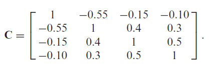
For this, I use the following API call to Portfolio Optimizer

    
	fetch('https://api.portfoliooptimizer.io/v1/assets/correlation/matrix/bounds', 
	      { 
		    method: 'POST',
		    headers: { 'Content-Type': 'application/json' },
            body: JSON.stringify({ assets: 4, 
			                       assetsCorrelationMatrix: [[1, -0.55, -0.15, -0.10], [-0.55, 1, 0.4, 0.3],[-0.15, 0.4, 1, 0.5], [-0.10, 0.3, 0.5, 1]],
                                   assetsGroup: [2,3,4]  
                                 }) 
          })    
    

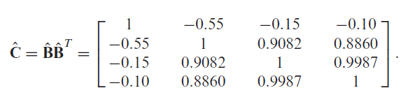
It returns the upper bounds correlation matrix

\[\approx \begin{pmatrix} 1 & -0.55 & -0.15 & -0.1 \newline -0.55 & 1 & 0.90821 & 0.88598 \newline -0.15 & 0.90821 & 1 & 0.99873 \newline -0.1 & 0.88598 & 0.99873 & 1 \end{pmatrix}\]

which corresponds to the matrix $\hat{C}$ computed by Numpacharoen and Bunwong³, as can be verified on Figure 2.

Figure 2. Example 2 from Numpacharoen and Bunwong. Upper bounds correlation matrix. Source: Numpacharoen and Bunwong

Computation of the lower bounds of a correlation matrix

Let $C \in \mathcal{M}(\mathbb{R}^{n \times n})$, $n \ge 3$, be a correlation matrix.

Suppose we would like to stress the correlations among a selected group of $2 \leq k \leq n-1$ assets to their minimum allowed values⁷ while keeping all the other correlations fixed.

By definition, the resulting correlation matrix will then be the lower bounds correlation matrix $L \in \mathcal{M}(\mathbb{R}^{n \times n})$ associated to the selected group of $k$ assets.

Notes:

• If there is no group of assets for which to keep the correlations fixed, the lower bounds matrix is then the equicorrelation matrix $C_{-\frac{1}{n-1}}$¹⁶.

Procedure

In the case $k = 2$, Numpacharoen and Bunwong³ propose to use the same procedure to compute the lower bounds matrix $L$ than to compute the upper bounds matrix $U$, the only change being at step 3, in which the correlative angles are stressed to $\pi$ instead of 0.

Unfortunately, in the case $k \geq 3$, there does not seem to be any published procedure to compute the lower bounds matrix $L$, because, as Numpacharoen and Bunwong³ put it:

it is much more difficult to create a matrix with many negative correlation coefficients compared to that with many positive correlation coefficients

Implementation in Portfolio Optimizer

A proprietary procedure is implemented in the Portfolio Optimizer endpoint /assets/correlation/matrix/bounds to compute the lower bounds of a correlation matrix.

Example of computation

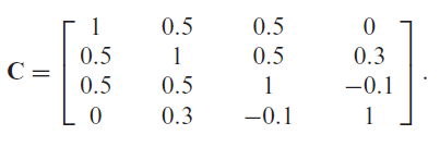
As an example of computation of the lower bounds of a correlation matrix, I will reproduce the example 1 of Numpacharoen and Bunwong³, in which the lower bounds of the correlation matrix displayed in Figure 3 are computed w.r.t. the last two assets

Figure 3. Example 1 from Numpacharoen and Bunwong. Asset correlation matrix. Source: Numpacharoen and Bunwong

For this, I use the following API call to Portfolio Optimizer

    
	fetch('https://api.portfoliooptimizer.io/v1/assets/correlation/matrix/bounds', 
	      { 
		    method: 'POST',
		    headers: { 'Content-Type': 'application/json' },
            body: JSON.stringify({ assets: 4, 
			                       assetsCorrelationMatrix: [[1, 0.5, 0.5, 0], [0.5, 1, 0.5, 0.3],[0.5, 0.5, 1, -0.1], [0, 0.3, -0.1, 1]],
                                   assetsGroup: [3,4]  
                                 }) 
          })    
    

It returns the lower bounds correlation matrix

\[\approx \begin{pmatrix} 1 & 0.5 & 0.5 & 0 \newline 0.5 & 1 & 0.5 & 0.3 \newline 0.5 & 0.5 & 1 & -0.66594 \newline 0 & 0.3 & -0.66594 & 1 \end{pmatrix}\]

which corresponds to the result mentioned in Numpacharoen and Bunwong³

Finally, the lower […] bounds of c4,3 and c3,4 are −0.6659 […].

Example of application - Sensitivity analysis of a risk parity portfolio

As a practical application of the shrinking method described in this post, I will now reproduce an example taken from Steiner¹⁹, which aims to conduct a sensitivity analysis of the volatility of a risk parity portfolio relative to one particular entry in the [asset] correlation matrix.

Computation of the initial risk parity portfolio weights

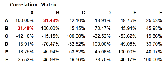
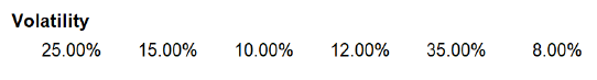
The asset correlation matrix $C_{ST}$ and the asset volatilities provided in Steiner¹⁹ are displayed in Figure 4 and in Figure 5.

Figure 4. Example from Steiner. Asset correlation matrix. Source: Steiner

Figure 5. Example from Steiner. Asset volatilities. Source: Steiner

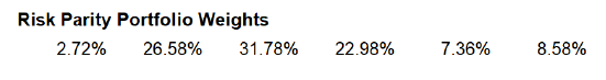
With these, and using the two Portfolio Optimizer endpoints

• /assets/covariance/matrix
• /portfolio/optimization/equal-risk-contributions

, the initial risk parity portfolio weights displayed in Figure 6 are computed.

Figure 6. Example from Steiner. Risk parity portfolio weights, computed with Portfolio Optimizer.

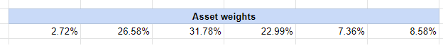
They are matching with the portfolio weights computed by Steiner¹⁹, displayed in Figure 7.

Figure 7. Example from Steiner. Risk parity portfolio weights. Source: Steiner

Computation of the lower and upper bounds of the asset correlation matrix

Steiner¹⁹ assumes that the correlation between [the first two assets] is of particular interest.

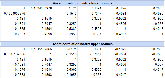
So, let’s compute the lower bounds and the upper bounds of the correlation matrix $C_{ST}$ w.r.t. the group of the first two assets.

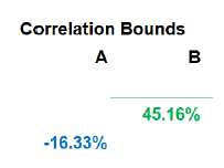
Using the Portfolio Optimizer endpoint /assets/correlation/matrix/bounds, this gives the two correlation matrices $L_{ST}$ and $U_{ST}$ displayed in Figure 8, which contain the same bounds for the correlation between the first two assets as those computed by Steiner¹⁹ displayed in Figure 9.

Figure 8. Example from Steiner. Bounds for the correlation between the first two assets, computed by Portfolio Optimizer.

Figure 9. Example from Steiner. Bounds for the correlation between the first two assets. Source: Steiner

Sensitivity analysis of the risk parity portfolio weights

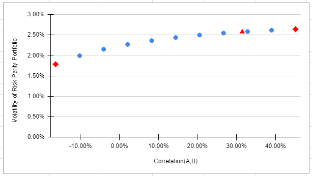
The lower and upper bounds correlation matrices $L_{ST}$ and $U_{ST}$ allow to analyze how the volatility of the risk parity portfolio evolves with the correlation between the first two assets thanks to the following procedure proposed by Steiner¹⁹:

• Compute several stressed correlation matrices of the form $ C_{ST, \lambda} = (1-\lambda) L_{ST} + \lambda U_{ST} $, with $\lambda \in [0,1]$²⁰
• For each of these stressed correlation matrices, compute the associated stressed risk parity portfolio weights
• For each of these stressed risk parity portfolio weights, compute the associated stressed portfolio volatility

Using the Portfolio Optimizer endpoints

• /assets/correlation/matrix/shrinkage
• /assets/covariance/matrix
• /portfolio/optimization/equal-risk-contributions
• /portfolio/analysis/volatility

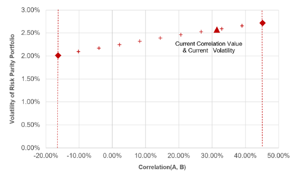
, this gives the portfolio volatility curve displayed in Figure 10, which approximately matches²¹ with the same curve taken from Steiner¹⁹ and displayed in Figure 11.

Figure 10. Example from Steiner. Sensitivity of the risk parity portfolio volatility to the correlation between the first two assets, computed with Portfolio Optimizer.

Figure 11. Example from Steiner. Sensitivity of the risk parity portfolio volatility to the correlation between the first two assets. Source: Steiner

Even more sensitivity analysis of the risk parity portfolio weights

Steiner¹⁹ concludes his example with the following remark:

We would, therefore, strongly recommend to supplement the sensitivity above analysis with a sensitivity analysis to changes in the average level of all correlations and possibly also selected blocks of the correlation matrix.

This second round of sensitivity analysis, although not illustrated in this post, is also perfectly doable with Portfolio Optimizer:

• A sensitivity analysis to changes in the average level of all correlations can be performed by shrinking the asset correlation matrix $C_{ST}$ toward the equicorrelation matrix $C_{1}$¹⁶
• A sensitivity analysis to changes in correlations within a selected block of the correlation matrix can be performed by shrinking the asset correlation matrix $C_{ST}$ toward its lower and upper bounds w.r.t. the selected block of $k \geq 3$ assets

Happy sensitivity analysis!

–

1. See Steiner, Andreas, Manipulating Valid Correlation Matrices. ↩

2. See Kawee Numpacharoen, Weighted Average Correlation Matrices Method for Correlation Stress Testing and Sensitivity Analysis, The Journal of Derivatives Nov 2013, 21 (2) 67-74. ↩ ↩²

3. See Kawee Numpacharoen & Kornkanok Bunwong (2013) Boundaries of Correlation Adjustment with Applications to Financial Risk Management, Applied Mathematical Finance, 20:4, 403-414. ↩ ↩² ↩³ ↩⁴ ↩⁵ ↩⁶ ↩⁷ ↩⁸ ↩⁹ ↩¹⁰

4. Positive semi-definite. ↩

5. See Stanley JC, Wang MD. Restrictions on the Possible Values of r12, Given r13 and r23. Educational and Psychological Measurement. 1969;29(3):579-581. ↩

6. Because it is a convex combination of two valid correlation matrices. ↩ ↩²

7. Ensuring that the stressed correlation matrix is a valid correlation matrix. ↩ ↩² ↩³

8. See P.H. Kupiec, Stress testing in a Value-at-Risk framework, Journal of Derivatives 6(1), (1998), pp. 7–24. ↩

9. See Riccardo Rebonato, Peter Jackel, The most general methodology to create a valid correlation matrix for risk management and option pricing purposes, Quantitative Research Centre of the NatWest Group, 135 Bishopsgate, EC2M 3UR. ↩

10. Also called hyperspherical parametrization, spherical parametrization, standard angles parameterization or triangular angles parameterization. ↩

11. See Riccardo Rebonato, Peter Jaeckel, The Most General Methodology to Create a Valid Correlation Matrix for Risk Management and Option Pricing Purposes. ↩ ↩²

12. See Rapisarda, F., Brigo, D. and Mercurio, F. (2007) Parameterizing correlations: a geometric interpretation, IMA Journal of Management Mathematics, 18(1), pp. 55–73. ↩ ↩² ↩³

13. See Mohsen Pourahmadi, Xiao Wang, Distribution of random correlation matrices: Hyperspherical parameterization of the Cholesky factor, Statistics & Probability Letters, Volume 106, 2015, Pages 5-12. ↩ ↩²

14. Of rank 1, so, positive semi-definite. ↩

15. Or one of its, if $C$ is positive semi-definite. ↩

16. See the blog post Correlation Matrix Stress Testing: Shrinkage Toward an Equicorrelation Matrix. ↩ ↩² ↩³

17. The exact order of the assets in the group does not matter. ↩

18. From the third property of the hypersphere decomposition, this will alter the correlation coefficients present in the lower right triangular part of the permuted correlation matrix $C_{\pi}$, and only them, which is exactly what is desired. ↩

19. See Steiner, Andreas, Upper and Lower Bounds for Entries in a Valid Correlation Matrix (June 23, 2021). ↩ ↩² ↩³ ↩⁴ ↩⁵ ↩⁶ ↩⁷ ↩⁸

20. From the figure in Steiner¹⁹, the exact number of such matrices seems to be equal to 11, with $\lambda$ taking the 11 values $0, \frac{1}{10}, …, 1$. ↩

21. The non-matches are located close to the extreme points, corresponding to the correlation matrices $L$ and $U$. ↩