Value-at-Risk Estimation: Improved Historical and Simulation-based Estimates with the Harrell-Davis Quantile Estimator

16 minute read

In a previous blog post of this series, the main univariate Value-at-Risk (VaR) estimation methods were described.

Among these, and for scenario-based VaR estimation like historical VaR or Monte Carlo VaR, the most widely used [non-parametric] estimator is the corresponding order statistic of the empirical quantile of the portfolio return distribution, or a linear combination of two subsequent order statistics¹.

Problem is, because they use too few sample elements¹, these estimators exhibit high variability and provides little information about the distribution of losses around the tail².

That problem is further exacerbated in a multivariate Value-at-Risk setting, under which these estimators might even yield inaccurate estimates³ of VaR sensitivities to portfolio positions (marginal VaR, component VaR…), irrespective of the number of scenarios used.

One possible solution is to use the Harrell-Davis quantile estimator⁴ instead, which is an estimator based on a weighted average of a range of order statistics³ substantially more efficient than the traditional estimators based on one or two order statistics⁴.

In this blog post, I will detail that quantile estimator and I will review its practical performances.

Reminders on Value-at-Risk

Value-at-Risk

The Value-at-Risk $VaR_{\alpha}$ of a portfolio over a time horizon $T$ (1 day, 10 days, 20 days…) and at a confidence level $\alpha$% $\in ]0,1[$ (95%, 97.5%, 99%…) can be defined as the opposite of the $1 - \alpha$ quantile of the portfolio return distribution over the time horizon $T$

\[\text{VaR}_{\alpha} = - F_X^{-1}(1 - \alpha)\]

, where:

$X$ is a random variable representing the portfolio return over the time horizon $T$
$F_X^{-1}$ is the inverse cumulative distribution function, also called the quantile function, of the random variable $X$

Univariate Value-at-Risk estimation through empirical quantile estimators

In a scenario-based approach to VaR estimation, whether relying on historical scenarios or simulated scenarios⁵, a sample of portfolio returns $r_1,…,r_n$ over a given time horizon $T$ is available.

The Value-at-Risk of that portfolio over the horizon $T$ at a confidence level $\alpha \in ]0,1[$ is then simply the opposite of the $(1 - \alpha)$% quantile of the empirical return distribution $r_1,…,r_n$, which essentially turns the problem of VaR estimation into a statistical quantile estimation problem³.

As noted in Akinshin¹, the traditional way to [estimate that $(1 - \alpha)$% quantile] is to use a single order statistic or a linear combination of two subsequent order statistics¹, although Hyndman and Fan⁶ actually describes nine types of traditional quantile estimators which are used in statistical computer packages¹.

For reference, with $r_{(1)} \leq r_{(2)} \leq … \leq r_{(n-1)} \leq r_{(n)}$ the order statistics of the sample of portfolio returns, the following two empirical portfolio VaR estimators, based on two traditional empirical quantile estimators, have been introduced in a previous blog post:

The opposite of the $\lfloor n (1 - \alpha) \rfloor + 1$-th highest portfolio return
\[\text{VaR}_{\alpha} = - r_{\left( \lfloor n (1 - \alpha) \rfloor + 1 \right)}\]
The linear interpolation between the opposite of the $\lfloor (n+1) \left( 1 - \alpha \right) \rfloor $-th and $ \lfloor (n+1) \left( 1 - \alpha \right) \rfloor + 1$-th highest portfolio returns
\[\text{VaR}_{\alpha} = - \left( 1 - \gamma \right) r_{\left( \lfloor (n+1) \left( 1 - \alpha \right) \rfloor \right)} - \gamma r_{\left( \lfloor (n+1) \left( 1 - \alpha \right) \rfloor + 1 \right)}\]
, with $\gamma$ $= (n+1) \left( 1 - \alpha \right)$ $- \lfloor (n+1) \left( 1 - \alpha \right) \rfloor$.

These two estimators are examples of non-parametric approaches to VaR estimation, because they do not make any specific distributional assumptions on the portfolio return distribution and they do not depend on any auxiliary parameter.

Value-at-Risk sensitivities

Beyond univariate VaR estimation, managing risk also requires the ability to identify the sources of risk and to assess the impacts of potential trades³.

For this, one must be able to evaluate the Value-at-Risk sensitivity to the positions that comprise a portfolio³, which is done thanks to the partial derivatives of VaR with respect to portfolio allocation⁷:

\[\text{MVaR}_{\alpha,i}(w) = \frac{\partial \text{VaR}_{\alpha} }{\partial w_i} (w)\]

, where

$m$ is the number of portfolio assets
$w \in [0,1]^{m}$ is the vector of portfolio asset weights
$\text{MVaR}_{\alpha,i}(w)$ is the partial derivative of the portfolio Value-at-Risk at a confidence level $\alpha$ with respect to the $i$-th asset of the portfolio, called the $i$-th marginal Value-at-Risk.

The properties of marginal VaRs are studied under general conditions in Hallerbach⁵ and in Gourieroux et al.⁷, which gives a slightly more explicit formula for marginal VaRs:

\[\text{MVaR}_{\alpha,i}(w) = - \Bbb{E} \lbrack X_i \vert X = - \text{VaR}_{\alpha}(w) \rbrack\]

, where $X_i$ is a random variable representing the $i$-th asset return over the time horizon $T$.

Multivariate Value-at-Risk sensitivities estimation through empirical quantile estimators

In a scenario-based approach to VaR estimation, marginal VaRs are typically estimated from either⁸:

One scenario⁹, in case the portfolio VaR is estimated through a single order statistic.
A linear combination of two subsequent scenarios, in case the portfolio VaR is estimated through a linear combination of two subsequent order statistics.

In more details, let $r^i_1,…,r^i_n$, $i=1..m$, be samples of the $m$ asset returns over the horizon $T$.

Then, from the formulas of the previous sub-sections:

In case the empirical portfolio VaR estimator is $\text{VaR}_{\alpha} = - r_{\left( \lfloor n (1 - \alpha) \rfloor + 1 \right)}$, the associated marginal VaRs are
\[\text{MVaR}_{\alpha,i} = - r^i_{\left[ \lfloor n (1 - \alpha) \rfloor + 1 \right)]}, i=1..m\]
, with $r^i_{[1]}, …, r^i_{[n]}$ the concomitants of the order statistics $r_{(1)}, …, r_{(n)}$.

For future reference, that approach to computing marginal VaRs is called scenario extraction in Epperlein and Smillie¹⁰.
In case the empirical portfolio VaR estimator is $\text{VaR}_{\alpha} = - \left( 1 - \gamma \right) r_{\left( \lfloor (n+1) \left( 1 - \alpha \right) \rfloor \right)} - \gamma r_{\left( \lfloor (n+1) \left( 1 - \alpha \right) \rfloor + 1 \right)}$, the associated marginal VaRs are
\[\text{MVaR}_{\alpha,i} = - \left( 1 - \gamma \right) r^i_{\left[ \lfloor (n+1) \left( 1 - \alpha \right) \rfloor \right]} - \gamma r^i_{\left[ \lfloor (n+1) \left( 1 - \alpha \right) \rfloor + 1 \right]}, i=1..m\]

Value-at-Risk estimation through the Harrell-Davis quantile estimator

As mentioned in the introduction, the main issue with the traditional empirical quantile estimators introduced in the previous section is that they experience a substantial lack of efficiency, caused by the variability of individual order statistics¹¹.

Additionally, Mausser³ notes that while the accurary of these estimators improves with increasing sample size, this is not necessarily true of the estimated quantile sensitivities³.

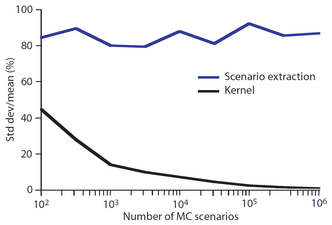
Such a puzzling behaviour¹² is illustrated in Figure 1 and is explained in Epperlein and Smillie¹⁰ as follows:

The reason for this is quite subtle: recall that [marginal Value-at-Risk] is defined as the [opposite of the] expectation of the component P&L, given that the parent P&L is equal to the [opposite of the] VaR.

Using [traditional empirical quantile estimators], one computes $-X_i \vert X = - \text{VaR}_{\alpha}(w)$, not $- \Bbb{E} \lbrack X_i \vert X = - \text{VaR}_{\alpha}(w) \rbrack$.

Thus, by using scenario extraction, we simply draw a single sample from a (conditional) probability distribution.

The distribution will have some variance, which we cannot expect to reduce simply by increasing the number of Monte Carlo runs.

Figure 1. Noise in marginal Value-at-Risk estimators as the number of Monte Carlo scenarios is increased, empirical quantile-based estimator (scenario extraction) v.s. kernel-based estimator. Source: Epperlein and Smillie.

In all cases, that behaviour is a huge limitation in terms of scenario-based marginal Value-at-Risk estimation…

L-estimators

Sheather and Marron¹¹ argues that an obvious way of improving the efficiency of sample quantiles is to reduce [their] variability by forming a weighted average of all of the order statistics, using an appropriate weight function¹¹.

Such a weighted average of order statistics, called an L-estimator, has a general form given by³:

\[Q_p(x) = \sum_{j=1}^n w_{p, n, j} x_{(j)}\]

, with:

$x_1, …, x_n$ the series of interest and $x_{(1)} \leq … \leq x_{(n)}$ the associated order statistics
$p \in [0,1]$ the $p$-th quantile of interest
$\sum_{j=1}^n w_{p, n, j} = 1$

To be noted that the empirical quantile estimators are examples of L-estimators, albeit ones that place the entire weights on at most two order statistics, so that the problem [with L-estimators] then becomes one of choosing¹³ the weight function¹¹ $w_{p, n, j}$.

The Harrell-Davis quantile estimator

The Harrell–Davis quantile estimator $HD_p$, introduced in Harrell and Davis⁴, is an L-estimator whose weights¹⁴ are related to the beta function:

\[HD_p(x) = \sum_{j=1}^n \left( I_{\frac{j}{n}}(a, b) - I_{\frac{j-1}{n}}(a, b) \right) x_{(j)}\]

, where:

$a = (n+1)p$
$b = (n+1)(1-p)$
$I_x(\alpha, \beta)$ is the regularized incomplete beta function

The typical shape of these weights is represented in Figure 2, which plots the weights for estimating the 0.95 quantile from a sample of 100 observations³.

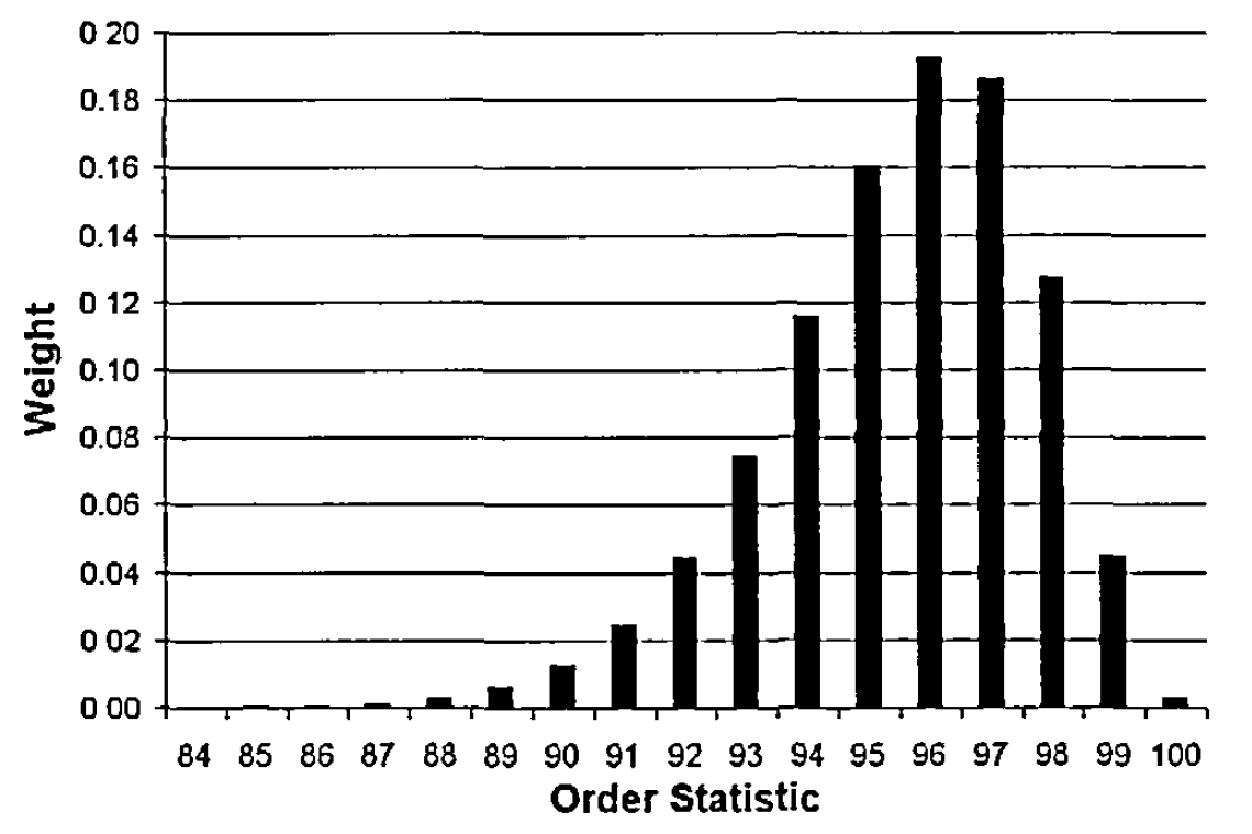
Figure 2. Harrell–Davis quantile estimator weights, p=0.95, n=100 observations. Source: Hausser.

On Figure 2, it is visible that the Harrell–Davis weights are distributed around a range of order statistics instead of being concentrated on at most two order statistics, which allows it to offer a significant gain in efficiency over the traditional [quantile estimators]⁴.

That gain in efficiency is empirically studied in Harrell and Davis⁴, which shows that - for small samples up to $n=60$ and over a wide variety of light- and heavy-tailed symmetric and asymmetric distributions⁴ - the Harrell–Davis quantile estimator is generally more than 10% as efficient as the traditional quantile estimator based on two order statistics.

Under a different experimental setup, Dielman et al.¹⁵ empirically establishes - for small samples up to $n=30$ and over misc. distributions -, that the Harrell–Davis quantile estimator is the overall best quantile estimator among 10 candidates, although it still has deficiencies concerning extreme percentile¹⁵.

That limitation¹⁶ is not surprising, though, with Harrell and Davis⁴ already mentioning that for some distributions like the exponential distribution, much higher sample sizes - $n \approx 80-100$ - may be required for $p = 0.9$ or above⁴.

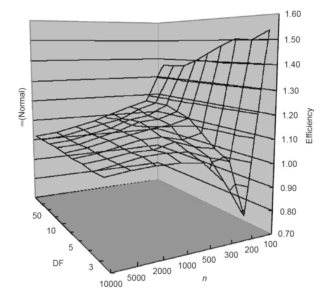
Under yet another experimental setup - this time for sample sizes ranging from $n=100$ to $n=10000$ and focused on fat-tailed Student-t distributions ,- Inui and Kijima¹⁷ concludes that the Harrell–Davis estimates are more efficient [than that of the ordinary empirical quantile] except in the case of t-distributions with $n \approx 200-300$ and [a degree of freedom] lower than 4¹⁷.

The exact gains in efficiency reported in Inui and Kijima¹⁷ are detailed in Figure 3.

Figure 3. Efficiency of the Harrell–Davis estimates v.s. the ordinary empirical quantile estimates for 99% confidence level, with varying sample size (n) and Student-t degree of freedom (DF). Source: Inui and Kijima.

Value-at-Risk and Value-at-Risk sensitivities estimation

In order to compute more robust risk analytics³ than with the empirical quantile estimators, Mausser³ proposes to use the Harrell–Davis quantile estimator for non-parametric Value-at-Risk and Value-at-Risk sensitivities estimation.

For this, Mausser³ defines:

The opposite of the Harrell–Davis $(1 - \alpha)$-th quantile estimator of the sample of portfolio returns $r_1,…,r_n$ as the Harrell–Davis portfolio VaR estimator
\[\text{VaR}_{\alpha} = - HD_{1 - \alpha}(r)\]
The opposite of the Harrell–Davis $(1 - \alpha)$-th concomitant estimator of the sample of asset returns $r^i_1,…,r^i_n$ as the Harrell–Davis $i$-th marginal VaR estimator, $i=1..m$
\[\text{MVaR}_{\alpha,i} = - \sum_{j=1}^n \left( I_{\frac{j}{n}}(a,b ) - I_{\frac{j-1}{n}}(a, b) \right) r^i_{[j]}\]
, where $a = (n+1)(1 - \alpha)$ and $b = (n+1)\alpha$.

That formula is derived in Mausser³, with the following comments in Bonollo et al.¹⁸:

The [marginal VaR] of each position is given by a weighted average of its P&Ls; the weights are given by the Harrell-Davis formula […], where the scenario with higher weight will be the VaR scenario of the portfolio.

For both estimators, the fact that VaR is calculated as a weighted combination of the losses across multiple scenarios has an inherent smoothing effect³.

This can be seen for example in Figure 4, which compares the Value-at-Risk trade risk profile³ obtained using the Harrell–Davis quantile estimator and the single-order statistic empirical quantile estimator.

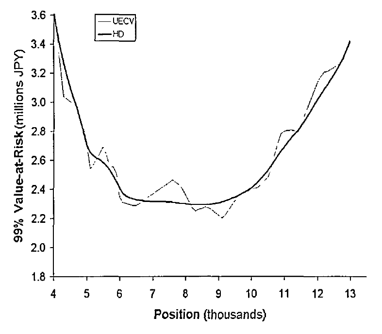
Figure 4. Harrell–Davis quantile estimator v.s. single order statistics empirical quantile estimator, 99% VaR trade risk profile for Mitsubushi EC 6mo 860 call. Source: Hausser.

That smoothness explains why the Harrell–Davis VaR estimator is more efficient than the single-order statistic based VaR estimator, with for example Bonollo and Mastrototaro¹⁹ reporting error estimates down by as much as 32 percentage points²⁰ in the context of default risk charge²¹ estimation, which is a Value-at-Risk at a 99.9% confidence level estimated over a 1 year horizon.

In the specific case of VaR sensitivies estimation, that smoothness also provides the Harrell–Davis marginal VaR estimator with the desirable property that, as the sample size increases, the standard deviation of the estimate decreases³, contrary to its empirical counterparts whose estimates variability not only exceeds that of the [Harrell–Davis] estimates, but actually gets larger as the sample size increases³, c.f. Figure 1.

That phenomenom is also reported in Bonollo et al.¹⁸, which observes that the [marginal] VaR obtained with Harrell-Davis weights is way more stable compared to the [empirical quantile-based] one¹⁸.

Comparison with other L-estimators

Several other Value-at-Risk estimators based on linear combinations of order statistics have been proposed in the litterature, among which:

The rectangular VaR estimator

That estimator, introduced in Hallerbach⁵ in the context of marginal Value-at-Risk estimation, is an equally-weighted average of all the order statistics in a neighborhood of the single-order statistic based empirical quantile estimator.
The triangular VaR estimator

That estimator, introduced in Epperlein and Smillie¹⁰ in the context of marginal Value-at-Risk estimation, is an L-estimator whose maximum weight is located at the index of the single-order statistic based empirical quantile estimator and whose weights are symmetrically decreasing to 0 at a selected rate from that maximum weight.
General kernel-smoothed VaR estimators

Those estimators, which effectively smooth the empirical distribution function by spreading each sample observation over an interval with a so-called kernel³ and of which the previous estimators are examples, are described in details in a previous blog post.

Compared to all these semi-parametric VaR estimators, one practical advantage of the Harrell-Davis VaR estimator is that it is fully non-parametric; that is, there are no parameters to choose (window size, kernel type, bandwidth…).

Another practical avantage, and maybe the most important one, is that its empirical performances are comparable to general kernel-smoothed VaR estimators:

Bonollo and Mastrototaro¹⁹ compares the Harrell-Davis estimator to the first two estimators and concludes that the best result was obtained with the Harrell-Davis estimator¹⁹.
Sheather and Marron¹¹ compares the Harrell-Davis estimator to an optimal Gaussian kernel-smoothed estimator and concludes that the former performs surprisingly well¹¹.

Incidentally, Sheather and Marron¹¹ demonstrates that the Harrell-Davis quantile estimator is asymptotically a Gaussian kernel estimator, although one whose bandwidth is in fact suboptimal¹¹ but often not too far from the optimum¹¹.

That suboptimality is an important feature of the Harrell-Davis quantile estimator, because general kernel-smoothed quantile estimators require the selection of a bandwidth parameter, which is typically done in a data-driven way.

Unfortunately, the choice of an optimal bandwidth is a difficult task, especially when smoothing the tails of underlying distributions with possible data scarcity²², so that a guaranteed suboptimality is probably more important in practice than a non-guaranteed optimality…

Caveats

Despite its very good performances, the Harrell-Davis quantile estimator also has some limitations to be aware of.

Bias

Inui and Kijima¹⁷ empirically shows that the Harrell–Davis estimator tends to have a more significant positive bias than the ordinary quantile estimator when used for fat-tail distributions¹⁷.

More precisely, and under a Monte Carlo simulation setting that uses Student-t distributions to model portfolio returns, Inui and Kijima¹⁷ demonstrates that:

The bias of both the Harrell–Davis VaR estimator and the ordinary quantile VaR estimator increases with higher confidence level $\alpha$, heavier tails for the portfolio returns and smaller sample size $n$.
The small sample bias ($n \approx 200$) of the Harrell–Davis VaR estimator is greater than that of the ordinary quantile VaR estimator for fat-tailed distributions with a degree of freedom lower than $\approx 6$.

Here, interestingly, the reverse is true for $n \approx 100$ and Inui and Kijima¹⁷ more generally states that the bias of the Harrell–Davis estimates of VaR with $n \approx 100$ is always smaller than that with $n \approx 200$, whatever the degree of freedom¹⁷.

That slightly higher²³ bias is not necessarily an issue, but because some empirical researches suggest to use [Student-t] distributions with [a degree of freedom] not greater than 4¹⁷ to model asset returns, it is a limitation of the Harrell–Davis VaR estimator to keep in mind.

As a side note, Kim and Hardy²⁴ argues that bias correction may increase the bias and substantially increase the rMSE²⁴ of bias-corrected VaR estimators, so that it is probably useless to try to improve the Harrell–Davis VaR estimator on this aspect.

Statistical robustness

Akinshin¹ highlights that the improved efficiency of the Harrell–Davis quantile estimator has a price¹ in that it becomes non robust in the statistical sense.

Indeed¹:

Since the estimation is a weighted sum of all order statistics with positive weights, a single corrupted element may spoil all the quantile estimations, including the median.

It may become a severe drawback in the case of heavy-tailed distributions in which it’s a typical situation when we have a few extremely large outliers.

For practical situations in which this non-robustness is an issue, Akinshin¹ proposes to use a trimmed modification of the Harrell-Davis quantile estimator¹ that is both more robust than the Harrell–Davis estimator […] and typically more statistically efficient than [the single-order statistic empirical estimator]¹.

The core idea of Akinshin’s¹ trimmed Harrell-Davis quantile estimator is to discard elements outside of the highest density interval of the underlying beta distribution¹ under the assumption that they might be contaminated.

This is done through the introduction of a parameter that needs to be carefully¹ selected - the width of the beta distribution highest density interval¹.

Nevertheless, in practice, determining that width parameter in the context of VaR estimation might prove to be difficult due to the extreme nature of the associated quantiles²⁵, so that the interested reader will probably need to perform some more analysis here.

Tail extrapolation

Like all L-estimators, the Harrell-Davis quantile estimator is limited by the fact that the estimated quantile cannot lie outside the range of the order statistics, which may be a concern when estimating extreme quantiles based on small samples³.

Hopefully, this is a well-known issue in VaR estimation with several alternative approaches readily available like extreme value theory-based VaR estimation.

Implementation in Portfolio Optimizer

Portfolio Optimizer implements the Harrell–Davis quantile estimator for both Value-at-Risk and Value-at-Risk contributions estimation, c.f. the documentation.

Conclusion

As Dielman et al.¹⁵ points out, there is not one [quantile] estimator that is always best; however, the results presented here do strongly argue in favor of [using the Harrell-Davis quantile estimator], in a wide range of cases¹⁵.

In the financial industry, this seems to be the choice made for example by Allianz France for their internal Solvency Capital Requirement (SCR) model, at least until April 2021²⁶.

So, why not giving it a try?

As usual, feel free to connect with me on LinkedIn or to follow me on Twitter.

–

See Andrey Akinshin (2022): Trimmed Harrell-Davis quantile estimator based on the highest density interval of the given width, Communications in Statistics - Simulation and Computation. ↩ ↩² ↩³ ↩⁴ ↩⁵ ↩⁶ ↩⁷ ↩⁸ ↩⁹ ↩¹⁰ ↩¹¹ ↩¹² ↩¹³ ↩¹⁴ ↩¹⁵
See Leszek Gadomski, Vasile Glavan, Expected shortfall and Harell-Davis estimators of value-at-risk, QUANTITATIVE METHODS IN ECONOMICS, Vol. XI, No. 1, 2010, pp. 81-89. ↩
See Mausser, H., 2001. Calculating quantile-based risk analytics with L-estimators. Algo Res. Quart. 4, 33–47. ↩ ↩² ↩³ ↩⁴ ↩⁵ ↩⁶ ↩⁷ ↩⁸ ↩⁹ ↩¹⁰ ↩¹¹ ↩¹² ↩¹³ ↩¹⁴ ↩¹⁵ ↩¹⁶ ↩¹⁷ ↩¹⁸ ↩¹⁹
See Harrell, F. E., and C. E. Davis. 1982. A new distribution-free quantile estimator. Biometrika 69 (3):635–40. ↩ ↩² ↩³ ↩⁴ ↩⁵ ↩⁶ ↩⁷ ↩⁸
See Winfried G. Hallerbach, Decomposing portfolio value-at-risk: a general analysis, Journal of Risk, volume 5, number 2 (winter 2002), pages: 1-18. ↩ ↩² ↩³
See Hyndman, R. J., & Fan, Y. (1996). Sample Quantiles in Statistical Packages. The American Statistician, 50(4), 361–365. ↩
See Gourieroux, C., Scaillet, O. and Laurent, J.P. (2000). Sensitivity analysis of Values at Risk. Journal of Empirical Finance, 7, 225-245. ↩ ↩²
Both of these approaches are non-parametric in nature. ↩
As noted in Mausser³, the marginal VaR for an instrument equals its per-unit loss in the particular scenario for which the portfolio loss equals the VaR³. ↩
See Epperlein, E., Smillie, A. Cracking VaR with kernels. RISK, 2006, vol. 9, pages 70-74. ↩ ↩² ↩³
See Sheather, Simon J., and J. S. Marron. “Kernel Quantile Estimators.” Journal of the American Statistical Association, vol. 85, no. 410, 1990, pp. 410–416. ↩ ↩² ↩³ ↩⁴ ↩⁵ ↩⁶ ↩⁷ ↩⁸ ↩⁹
Mausser³ also notes that such a weird behaviour tends to occur whenever an instrument’s losses do not relate with those of the portfolio in a consistent manner³. ↩
When the weight function is properly chosen, L-estimators exhibit certain desirable asymptotic properties such as asymptotic normality (under very general conditions)¹⁵ - which facilitates the construction of confidence intervals for the quantile³ - and compete favorably with M estimators¹⁵. ↩
For practical applications, it is worth noting that the Harrell–Davis weights depend only on the sample size $n$ and on the quantile $q$. ↩
See Dielman, T., Lowry, C., Pfaffenberger, R., 1994. A comparison of quantile estimators. Comm. Statist.: Simulation Comput. 23, 203–228. ↩ ↩² ↩³ ↩⁴ ↩⁵ ↩⁶
Another limitation is that since the Harrell–Davis quantile estimator requires evaluation of the incomplete beta function, this estimator cannot be computed over ranges of values for which the incomplete beta function is undefined¹⁵, which is the case for small $n$ and very small $p$. ↩
See Koji Inui, Masaaki Kijima, Atsushi Kitano, VaR is subject to a significant positive bias, Statistics & Probability Letters, Volume 72, Issue 4, 2005, Pages 299-311. ↩ ↩² ↩³ ↩⁴ ↩⁵ ↩⁶ ↩⁷ ↩⁸ ↩⁹
See Michele Bonollo, Giacomo Colombo, Giacomo Giannoni and Antonio Menegon, Risk Attribution, iason, Research Paper Series, N.48, 05/07/2022. ↩ ↩² ↩³
See Michele Bonollo and Leonardo Mastrototaro, A Comparison of Advanced Methods for the Quantile Estimation in the Risk Management Field, iason, Research Paper Series, N.80, 07/10/2025. ↩ ↩² ↩³
From 73.2% to 41.2% (3rd case of $n = 1000$ in Table 1), c.f. Bonollo and Mastrototaro¹⁹. ↩
The default risk charge (DRC) is a regulatory measure designed to capture default risk within the trading portfolio, as required by Basel standards¹⁹. ↩
See Keming Yu & Abdallah K. Ally & Shanchao Yang & David J. Hand, Kernel quantile based estimation of expected shortfall, Journal of Risk, Journal of Risk. ↩
The bias of the Harrell–Davis VaR estimator seems to be greater by about 5 percentage point (19% v.s. 14%) for a Student-t distribution with a degree of freedom equal to 3, c.f. Figure 6 of Inui and Kijima¹⁷. ↩
See Kim JHT, Hardy MR. Quantifying and Correcting the Bias in Estimated Risk Measures. ASTIN Bulletin. 2007;37(2):365-386. ↩ ↩²
Especially at very high confidence levels $\alpha=99$%, $\alpha=99.5$%, … ↩
See IBAZIZEN Rachid, Creation d’un cadre prudentiel pour le pilotage d’un FRPS de grande taille, Memoire. ↩