The Turbulence Index: Measuring Financial Risk

One of the challenges in portfolio management is the timely detection of financial market stress periods, typically characterized by an increase in volatility and a breakdown in asset correlations¹.

Chow et al.² propose to detect such periods through the usage of the caste distance, a measure initially introduced by Mahalanobis³⁴ to classify human skulls in India and now commonly called the Mahalanobis distance.

Kritzman and Li⁵, who label this measure the turbulence index, establish its empirical properties and illustrate some of its possible applications in portfolio management.

In this post, I will show how to compute a turbulence index for global financial markets and how this turbulence index could be used to scale the market exposure of a portfolio of U.S. equities.

Mathematical preliminaries

Definition

Let be:

• $n$, the number of assets in a given universe of assets
• $\mu_{t’} \in \mathbb{R}^{n}$, the vector of the average asset returns over an historical reference period $t’$
• $\Sigma_{t’} \in \mathcal{M}(\mathbb{R}^{n \times n})$, the asset covariance matrix over an historical reference period $t’$
• $r_t \in \mathbb{R}^{n}$, the vector of the asset returns over a period $t \ne t’$

The turbulence index $d_t$ for the universe of assets over the period $t$ is defined as the following squared and normalized Mahalanobis distance⁶:

\[d_t = \frac{1}{n} (r_t - \mu_{t'}) {}^t \Sigma{_{t'}}^{-1} (r_t - \mu_{t'})\]

Less formally, as Marc Kritzman puts it⁷:

[The] Turbulence [Index] is a measure of statistical unusualness that takes into account both the magnitude of returns and how they interact with one another.

Interpretation

The turbulence index quantifies the degree of unusual behavior within a given universe of assets.

The intuition behind it is that the more asset returns, volatilities and correlations differ from their historical norms, the more likely it is that these differences result from a significant market event⁸ rather than from random noise.

Mathematical properties

The turbulence index inherits all the mathematical properties of the squared Mahalanobis distance, up to the normalizing constant $1/n$.

For example:

Property 1: The turbulence index is an appropriate measure of multivariate distance for elliptically distributed asset returns, which includes multivariate normal, Student’s t and Cauchy distributions⁹.

Property 2: The turbulence index is invariant under affine transformations of the asset returns¹⁰.

Other properties, and in particular the relationship of the turbulence index with the chi-squared distribution, can be found in Stockl et al.¹⁰ and in Kritzman et al.¹¹.

Empirical properties

Kritzman and Li⁵ establish several empirical properties of the turbulence index.

For example:

• It tends to spike during identifiable periods of financial market stress like the 1987 Black Monday, the Gulf War or the Global Financial Crisis
• It tends to remain elevated for a couple of weeks after an initial spike¹²

Global financial markets turbulence index

I will now show how to compute a turbulence index for global financial markets, using the Portfolio Optimizer API.

Similar to Kritzman and Li⁵, I will use (weekly) returns data for the following seven¹³ global asset classes:

Asset Class
U.S. Stocks
Non-U.S. Stocks
U.S. Bonds
Non-U.S. Bonds
U.S. Real Estate
Non-U.S. Real Estate
Commodities

Contrary to Kritzman and Li⁵, though, I will not compute the average asset returns and the asset covariance matrix over the full returns data sample, but I will use a rolling window approach instead.

This change is important to avoid any look-ahead bias, i.e., to demonstrate that the turbulence index is capable of detecting periods of financial market stress using only data available up to that point in time.

The methodology to compute this turbulence index is the following.

At the end of each week:

• The mean asset returns $\mu$ are computed over a window of past returns data¹⁴, using the Portfolio Optimizer endpoint /assets/returns/mean
• The asset sample covariance matrix $\Sigma$ is computed over a window of past returns data, using the Portfolio Optimizer endpoint /assets/covariance/matrix
• The latest asset returns $r$ are extracted
• The turbulence index for the seven assets is computed, using the Portfolio Optimizer endpoint /assets/analysis/turbulence-index with $\mu$, $\Sigma$ and $r$

The resulting turbulence index over the period April 2009 - March 2022¹⁵ is illustrated in figure 1, on which four financial crisis are also labeled.

Figure 1. Turbulence index of seven global asset classes, April 2009 - March 2022

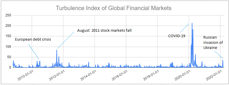
It is clear that:

• The turbulence index tends to spike during identifiable periods of financial market stress: the European debt crisis, the August 2011 stock markets fall, the COVID-19 pandemic, the Russian invasion of Ukraine…
• The turbulence index tends to remain elevated for a couple of weeks after an initial spike

So, the turbulence index seems to demonstrate the same empirical properties over the period 2009 - 2022 as those established in Kritzman and Li⁵ over the period 1980 - 2009 about 12 years ago.

I personally find that this is some pretty amazing out-of-sample robustness!

Example of usage - Scaling the market exposure of a portfolio

Equipped with a turbulence index for global financial markets, the next step is to investigate how to integrate it into a portfolio risk management process.

In particular, knowing that periods of elevated turbulence index tend to correspond to periods of lower than usual asset returns⁵, it might be possible to enhance a portfolio risk-return profile by de-risking upon spikes in the turbulence index.

This idea was already explored in Kritzman and Li⁵, who proposed to scale the market exposure of a foreign exchange carry strategy in inverse proportion of a turbulence index for G–10 currencies.

I propose to revisit this idea, this time to scale the market exposure of a portfolio of U.S. equities.

The strategy is the following.

At the end of each week:

• Compute the value of the global financial markets turbulence index defined in the previous paragraph
• Determine how elevated is this turbulence index relative to its history¹⁶, on a scale $s$ from 0% to 100%
• Allocate $s$% of the portfolio to cash and $1-s$% of the portfolio to U.S. equities

Figure 2 illustrates this strategy with the SPY ETF (U.S. equities) and the SHY ETF (cash) over the period April 2009 - March 2022, and compare it to a buy and hold strategy over the same period.

Figure 2. Buy and hold v.s. turbulence-adjusted SPY

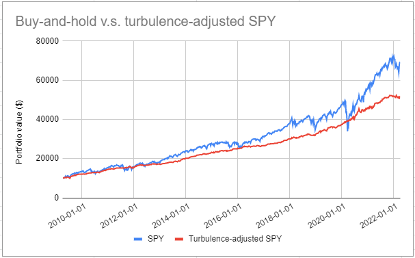
Visually, it appears that this strategy seems to be efficient in managing risk.

Figures confirm this:

Portfolio Management Strategy	Average Exposure	Annualized Sharpe Ratio	Maximum (Weekly) Drawdown
Buy and hold	100%	~1	~32%
Turbulence-adjusted	~50%	~2.20	~6%

Now, this strategy is not a silver bullet.

For example, it is not able to keep up with an extreme bull market, like the violent recovery which took place after the COVID-19 crisis.

But it definitely seems to do a very good job in protecting a portfolio in periods of market turbulence!

Conclusion

More than 20 years after its introduction in the context of financial markets, the Mahalanobis distance has proved to be a useful financial risk indicator in the form of the turbulence index.

For the interested readers, research on the Mahalanobis distance in another financial context is on-going at this date, with a recent paper on using it to construct a business cycle indicator¹¹.

Long live the Mahalanobis distance!

–

1. For example, correlations between assets tend to increase during crises, c.f. Sebastien Page & Robert A. Panariello (2018) When Diversification Fails, Financial Analysts Journal, 74:3, 19-32 and references therein. ↩

2. See George Chow, Jacquier, E., Kritzman, M., & Kenneth Lowry. (1999). Optimal Portfolios in Good Times and Bad. Financial Analysts Journal, 55(3), 65–73.. ↩

3. See Mahalanobis, P.C., 1927; Analysis of race mixture in Bengal, Journal and Proceedings of the Asiatic Society of Bengal, 23:301–333. ↩

4. See Mahalanobis, P.C., 1936, On the generalized distance in statistics. Proceedings of the National Institute of Sciences of India, 2, 49-55. ↩

5. See M. Kritzman, Y. Li, Skulls, Financial Turbulence, and Risk Management,Financial Analysts Journal, Volume 66, Number 5, Pages 30-41, Year 2010. ↩ ↩² ↩³ ↩⁴ ↩⁵ ↩⁶ ↩⁷

6. See Kinlaw, W., Turkington, D. Correlation surprise. J Asset Manag 14, 385–399 (2013). ↩

7. See Susan B. Weiner, Turbulence Can Improve Portfolio Diversification, August 18, 2009. ↩

8. Such a significant market event usually being a financial market stress… ↩

9. See Ann F. S. Mitchell, & Krzanowski, W. J. (1985). The Mahalanobis Distance and Elliptic Distributions. Biometrika, 72(2), 464–467. ↩

10. See Stockl, S., Hanke, M. Financial Applications of the Mahalanobis Distance. Applied Economics and Finance, [S.l.], v. 1, n. 2, p. 78-84, oct. 2014. ↩ ↩²

11. See W. Kinlaw, M. Kritzman, and D. Turkington, A new index of the business cycle, Journal Of Investment Management, Vol. 19, No. 3, (2021), pp. 4–19. ↩ ↩²

12. In other words, it is persistent. ↩

13. Compared to Kritzman and Li⁵, I included the additional asset class Non-U.S. Real Estate to be consistent with the other asset classes. ↩

14. The exact size of this window does not seem to heavily influence the computation of the turbulence index, with anything from six months to several years giving more or less the same results. ↩

15. Kritzman and Li⁵ illustrate their article with asset returns over the period January 1980 – April 2009, so that I chose to use asset returns starting from April 2009 as an out-of-sample test. ↩

16. I will not disclose my implementation details for this step, but using the quintiles approach of Kritzman and Li⁵ gives similar results. ↩