The Modified Gerber Statistic: A Threshold-free Co-Movement Statistic for Covariance Estimation and Portfolio Construction

A previous blog post described the Gerber statistic¹, a measure of co-movement introduced in Gerber et al.¹ built upon the idea of excluding small return observations deemed to be noise and of estimating dependence using a function robust to outliers².

Since its publication, different improvements to that statistic have been suggested in the litterature (Smyth and Broby³, Flint and Polakow²), which has led to the development of the modified Gerber statistic⁴ in Gerber et al.⁴.

In this blog post post, I will detail the construction of the modified Gerber statistic, show how it overcomes the main limitations of the original Gerber statistic and finally discuss some of its practical aspects (behaviour against the full sample correlation in case of joint normal returns, non-positive-semidefiniteness of the associated correlation matrix…).

As an example of usage, I will compare the two flavors of the Gerber statistic in the context of the multi-asset class portfolio investment strategy described in Gerber et al.¹.

Mathematical preliminaries

The Gerber statistic

The Gerber statistic is discussed elsewhere on this blog.

The modified Gerber statistic

Definition

Let be two assets $i$ and $j$ whose returns $r_{i,t}$ and $r_{j,t}$, $t=1..T$, have been observed over $T$ time periods.

The modified Gerber statistic $\text{MGS}_{ij}$ of these two assets is computed as follows⁴:

• Each asset return $r_{i,t}$ and $r_{j,t}$, $t=1..T$, is first converted to a centered percentile.

  This is done through the transformation

  \[u_{k,t} = \widehat{F}_{k,t}(r_{k,t}) - 0.5, k=i,j, t = 1,...,T\]

  , where $\widehat{F}_{k,t}$ denotes the within-window empirical percentile-rank transform, using average ranks for tied observation⁴, for the asset $k=i,j$.

• Then, each centered percentile pair $\left( u_{i,t}, u_{j,t} \right)$, $t = 1,…,T$, is weighted by a function $w_{ij,t}$.

  That function is equal to

  \[w_{ij,t} = \left( \frac{ \sqrt{(1+|u_{i,t}|)(1+|u_{j,t}|)} }{ 1 + \left||u_{i,t}| - |u_{j,t}|\right|^\eta } \right)^\gamma\]

  , where:

  • $\eta > 0$ is a penalty parameter controlling how quickly the weights decrease when centered percentiles of asset returns diverge, with larger $n$ reducing that penalty for every nonzero mismatch⁴ and therefore more permissive of one-sided observations⁴
  • $\gamma > 0$ is a curvature parameter that controls overall contrast⁴, with values above one amplifying differences between already high- and low-weight observations⁴ and values between zero and one flattening them⁴.

• Finally, the modified Gerber statistic $\text{MGS}_{ij}$ is obtained by a weighted sum⁵ involving the sign of the product of the centered percentiles $u_{i,t}$ and $u_{j,t}$.

  The exact formula is:

  \[\text{MGS}_{ij} = \frac{ \sum_{s=1}^{T} \operatorname{sign}(u_{i,t} u_{j,t})\,w_{ij,t}}{ \sum_{t=1}^{T} w_{ij,t}}\]

  As a side note, Gerber et al.⁴ additionally describes a decayed modified Gerber statistic which is obtained by a temporally weighted sum, with formula:

  \[\text{MGS}_{ij}^h = \frac{ \sum_{s=1}^{T} d_t(h) \operatorname{sign}(u_{i,t} u_{j,t})\,w_{ij,t}}{ \sum_{t=1}^{T} d_t(h) w_{ij,t}}\]

  , where $d_t(h) = 2^{-(T-t)/h}$ with $h > 0$ a half-life parameter.

Rationale

The modified Gerber statistic aims to overcome some practical limitations of the original Gerber statistic:

• The reliance on non-standardized asset returns

  Smyth and Broby³ reminds that the definition of the original Gerber statistic involves a region in the scatter plot of the asset joint returns⁶ - called the $NN$ subset in Gerber et al.¹ - in which it is difficult to ascertain if co-movement is evidence of underlying connection or simply noise³.

  Problem is, for returns distributions with non-zero means and different widths³ it turns out that this region is actually different from the $NN$ subset³!

  As a solution to that problem, Gerber et al.⁴ choses to use the non-parametric percentile transformation $u$, which put equities, bonds, gold, REITs, and commodities on a common scale before co-movement is estimated⁴.

  Compared to the simpler zero mean/unit standard deviation standardization suggested in Smyth and Broby³, that choice allows to limit the influence of extreme raw values⁴.

• The need to select a threshold

  Gerber et al.⁴ highlights that the original Gerber statistic involves the selection of a threshold that defines a meaningful event⁴, thus leading to a cutoff problem⁴ because an observation just below the threshold is fully ignored, while one just above it [is fully taken into account]⁴.

  In addition, due to the nature of that statistic, it is very difficult to know a priori how [it] will behave as one changes the conditioning threshold²…

  As a consequence, Gerber et al.⁴ defines the modified Gerber statistic without reference to any threshold, thereby removing an avoidable source of specification risk⁴ and making it more practitioner-oriented⁴.

  This is made possible by the usage of the continuous weighting function $w$.

• The discarding of magnitude information

  The original Gerber statistic discards information about the magnitude of asset returns beyond the threshold.

  Smyth and Broby³ explains how this might be detrimental for the purposes of co-movement analyses³:

  To illustrate, consider two uncorrelated stocks.

  A simultaneous co-movement of two standard deviations is much less likely than a simultaneous co-movement of one standard deviation.

  The situation changes when stocks are correlated, however, the former is still less likely than the latter.

  When the former occurs, therefore, we should consider it as having greater evidential value in the case for connection than the latter.

  In order to give the most influence to episodes in which both assets occupy similarly unusual states and less influence to one-sided events⁴, and in the spirit of Flint and Polakow², Gerber et al.⁴ proposes to use the flexible weighting and dependence function² $w$ as a replacement for the binary weighting function used in the original Gerber statistic.

The modified Gerber correlation matrix

Let be:

• $n$, the number of assets in a universe of assets
• $r_{i,1},…,r_{i,T}$, the return of the asset $i=1..n$ over each time period $t=1..T$

The modified Gerber asset correlation matrix $mG \in \mathcal{M}(\mathbb{R}^{n \times n})$ is then defined by:

\[mG_{i,j} = \text{MGS}_{ij}, i=1..n, j=1..n\]

, where $\text{MGS}_{ij}$ is the modified Gerber statistic between asset $i$ and asset $j$.

At this point, one important remark is that $mG$ might not be a valid correlation matrix.

Indeed, Gerber et al.⁴ emphasises that there is no theoretical guarantee that the modified Gerber asset correlation matrix is positive-semidefinite.

More on this later.

The modified Gerber covariance matrix

Let be:

• $n$, the number of assets in a universe of assets
• $mG \in \mathcal{M}(\mathbb{R}^{n \times n})$ , the modified Gerber asset correlation matrix
• $\sigma_1,…,\sigma_n$, the asset standard deviations

The modified Gerber asset covariance matrix $\Sigma_{mG} \in \mathcal{M}(\mathbb{R}^{n \times n})$ is then defined by:

\[\left( \Sigma_{mG} \right)_{i,j} = mG_{i,j} \, \sigma_i \, \sigma_j, i=1..n, j=1..n\]

As in the previous sub-section, one important remark is that $\Sigma_{mG}$ might not be a valid covariance matrix due to the lack of positive-semidefiniteness of the underlying modified Gerber asset correlation matrix.

Practical considerations

Influence of the parameters $\eta$ and $\gamma$

While the modified Gerber statistic is threshold-free, it is not parameter-free, with both the penalty parameter $\eta$ and the curvature parameter $\gamma$ to choose.

For these:

• Gerber et al.⁴ proposes to use the default values $\eta = 1$ and $\gamma = 1$.
• Smyth and Broby³ proposes to use - for a weighting function slightly different from the one described in Gerber et al.⁴ - the intuitively appealing $\eta = 2$³ because that parameter is related to a one-dimensional Manhattan distance where the components are magnitudes of standardized returns³ and $\gamma = 1$.

In any cases, it is interesting to understand the influence of these two parameters on the modified Gerber statistic.

For this, I will re-use the methodology described in Flint and Polakow² to compute correlation profiles⁷ for the modified Gerber statistic.

That methodology⁸ relies on a simple two-asset simulation framework [assuming joint normal returns], controlling the asset means and volatilities and imposing a fixed unconditional (full-sample) correlation².

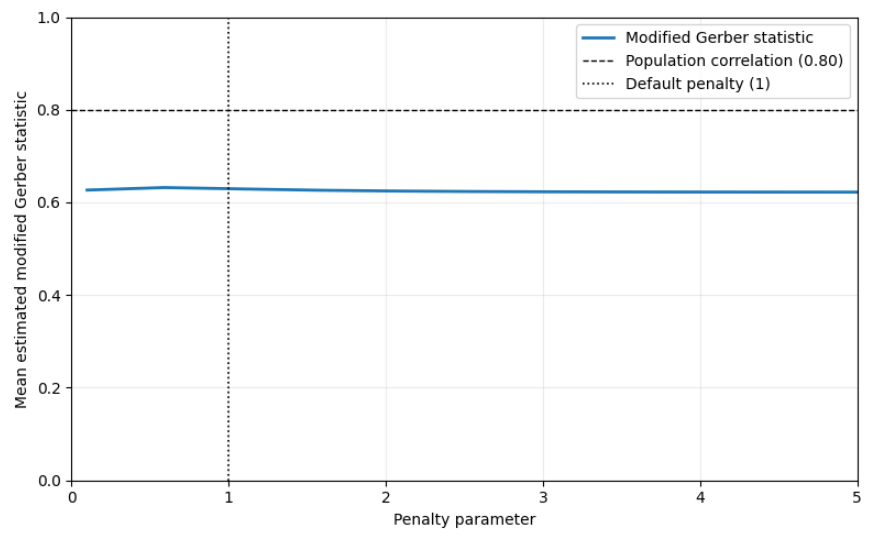
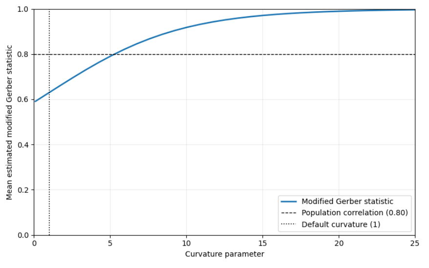
Figure 1 and Figure 2 depict the correlation profile obtained by simulating $T = 10 000$ return pairs per estimated correlation profile, with the modified Gerber statistic averaged across 50 runs.

Figure 1. Correlation profile of the modified Gerber statistic versus penalty parameter for a joint normal market with unconditional correlation of 0.80 (dashed horizontal line), curvature parameter fixed to 1.

Figure 2. Correlation profile of the modified Gerber statistic versus curvature parameter for a joint normal market with unconditional correlation of 0.80 (dashed horizontal line), penalty parameter fixed to 1.

From these figures, it seems that:

• The penalty parameter $\eta$ does not influence a lot the modified Gerber statistic.

  This confirms the results of Gerber et al.⁴, in which $\eta$ is varied from 1 to 5 with no meaningful impact⁹ on test results.

• The curvature parameter $\gamma$ has a much more pronounced influence on the modified Gerber statistic, with the resulting correlation equal to 1 for all practical purposes starting from $\gamma \approx 15$.

  As a side note, the correlation profile depicted in Figure 2 seems to behave similarly to the correlation profile of one¹⁰ of the Gerber statistics illustrated in Flint and Polakow².

Influence of the unconditional correlation

Following Flint and Polakow², another interesting question to ask is what happens to the [modified Gerber statistic] profiles when the unconditional (full-sample) correlation is varied².

Using the same methodology as in the previous sub-section, but this time varying the unconditional correlation from -1 to 1 while keeping the penalty and the curvature parameters fixed to 1, results are depicted in Figure 3.

Figure 3. Correlation profile of the original and modified Gerber statistics as a function of unconditional (full-sample) correlation.

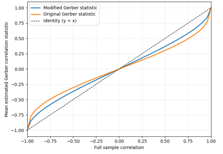
Figure 3 highlights that, like its original counterpart to which it is compared¹¹, the modified Gerber statistic seems to consistently pull the unconditional correlation towards zero², although with a slightly lower intensity.

Influence of the number of observations

Again following Flint and Polakow², and because in a practical asset allocation setting, sample sizes are likely to be several orders of magnitude smaller than [$T = 10 000$] observations², it is imperative to understand just how sensitive [the modified Gerber statistic] is to sample size².

For this, I generated 500 different samples of $T = 36$¹² joint normal asset returns with an unconditional correlation of 0.60, and the boxplot of the 500 associated modified Gerber statistics is represented in Figure 4.

Figure 4. Boxplot of the modified Gerber statistic with penalty and curvature parameters fixed to 1 for 500 joint normal samples of size T = 36 with unconditional correlation of 0.60.

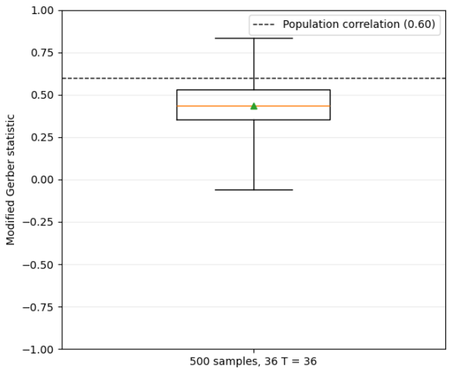
From Figure 4, it appears that there is considerable variation in the [modified Gerber statistic] when estimated with limited observations², which empirically demonstrates that the modified Gerber statistic inherits¹³ the variability of its parent mentioned in Flint and Polakow².

Positive-semidefiniteness of the modified Gerber correlation matrix

As already mentioned in the previous section, the modified Gerber correlation matrix is not guaranteed to be positive-semidefinite in theory.

How frequent is that lack of positive semi-definiteness in practice?

In order to answer that question, I propose to use the following procedure:

• Draw at random¹⁴ a given number of asset returns within a universe of assets
• Compute the associated modified Gerber correlation matrix
• Check whether it is positive-semidefinite¹⁵
• Repeat

Figure 5 illustrates the results obtained when using that procedure with:

• The universe of 9 assets already used in Gerber et al.¹ and made of monthly returns over the period January 1988 - December 2020 for:
  • US large cap stocks, represented by the S&P 500 index
  • US small cap stocks, represented by the Russell 2000 index
  • Developed markets ex. US and Canada large and mid cap stocks, represented by the MSCI EAFE index
  • Emerging markets large and mid cap stocks, represented by the MSCI Emerging Markets index
  • US treasuries, government-related and corporate bonds, represented by the Bloomberg Barclays US Aggregate Bond index
  • US high yield corporate bonds, represented by the Bloomberg Barclays US Corporate High Yield Bond index
  • US real estate, represented by the FTSE NAREIT all equity REITS index
  • Gold
  • Commodities, represented by the S&P GSCI Goldman Sachs Commodity index

• A number of drawn asset returns ranging from 6 to 54

  This range allows to cover all the situations from less observations than the number of assets $\left( \frac{T}{n} < 1 \right)$ to much more observations than the number of assets $\left( \frac{T}{n} = 6 \right)$.

• A number of 1000 random draws of asset returns per given number of drawn asset returns

Figure 5. Positive-semidefiniteness frequency of the modified Gerber correlation matrix, multi asset-classes universe of 9 assets.

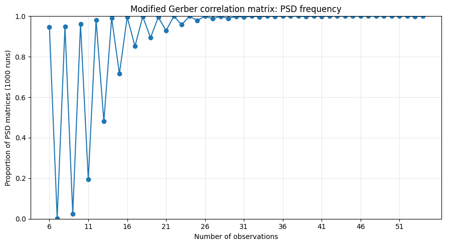
A couple of comments on Figure 5¹⁶:

• In general, the more observations, the most “certain” the positive-semidefiniteness of the modified Gerber correlation matrix.

  But this is without guarantees, with for example 29 or 31 observations still leading to a few non-positive-semidefinite modified Gerber correlation matrices.

• Nevertheless, 2 different patterns of positive-semidefiniteness seem to exist, for an odd v.s. an even number of observations.

  In particular, using an even¹⁷ number of observations seems to drastically increase the proportion of modified Gerber correlation matrices that are positive-semidefinite, especially when that number of observations is low compared to the number of assets.

  I have no explanation for this phenomenon, but interested readers are certainly encouraged to dig deeper!

• Starting from $T = 4n$, it seems that the modified Gerber correlation matrix can be considered as positive-semidefinite, whether $n$ is even or odd.

All in all, Figure 5 confirms that production use [of the modified Gerber correlation matrix] also requires […] positive-semidefinite validation or repair of the final matrix⁴, especially if the number of observations $T$ is not enforceable.

Hopefully, repair mechanisms for non-positive-semidefinite correlation matrices are well know, among which the computation of the nearest correlation matrix.

Implementation in Portfolio Optimizer

Portfolio Optimizer implements two endpoints related to the modified Gerber statistic:

• /assets/correlation/matrix/estimation/gerber/modified, to compute the modified Gerber correlation matrix
• /assets/covariance/matrix/estimation/gerber/modified, to compute the modified Gerber covariance matrix

Example of usage - empirical performances

Gerber et al.⁴ studies the empirical performances of the modified Gerber covariance matrix under a long-only target-risk mean-variance framework⁴ using 2 different universes of assets:

• A universe of 10 internationally diversified assets
• A universe of U.S. large stocks (S&P 500)

In this blog post, and for consistency with the previous blog post on the original Gerber statistic, I propose to revisit the original study of Gerber et al.¹ that uses the universe of 9 assets introduced in a previous section.

In details, I will backtest the following portfolio investment strategy over the period January 1988 - December 2020:

1. At the end of each month, compute mean-variance input estimates over the past 24 months of returns
   • The average return vector $\mu = \left( \mu_{SPX},…,\mu_{SPGSCI} \right)$
   • The sample covariance matrix $\Sigma$
   • The original Gerber covariance matrix $\Sigma_{G}$, with a Gerber threshold equal to 0.5
   • The modified Gerber covariance matrix $\Sigma_{mG}$, with both penalty and curvature parameters equal to 1
2. Then, compute no-short-sales constrained mean-variance efficient portfolios with an annualized volatility target of 3%, 5%, …, 15%
   • Using $\mu$ and $\Sigma$
   • Using $\mu$ and $\Sigma_{G}$
   • Using $\mu$ and $\Sigma_{mG}$

Figure 6 depicts the resulting three ex post mean-variance efficient frontiers.

Figure 6. Nine-asset universe, ex post mean-variance efficient frontiers, January 1990 - December 2020.

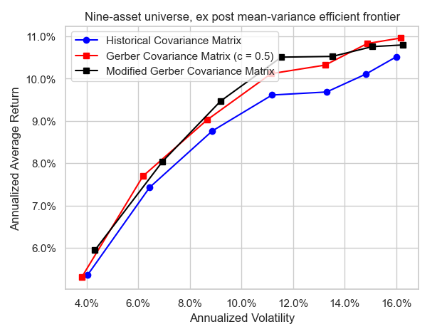
On Figure 6, it is visible that:

• The efficient frontiers corresponding to the two Gerber covariance matrices both dominate the efficient frontier corresponding to the historical covariance matrix.
• The efficient frontier corresponding to the modified Gerber covariance matrix dominates the efficient frontier corresponding to the original Gerber covariance matrix for an annualized portfolio volatility ranging from 7% to 14%.

The last point makes the modified Gerber covariance matrix especially interesting compared to its original counterpart, because that range of portfolio volatility matches with the range of portfolio volatility usually encountered in practice for multi-asset class portfolios.

Conclusion

I hope that thanks to this blog post you now have a better understanding of the modified Gerber statistic.

For more analyses like this one, feel free to connect with me on LinkedIn or to follow me on Twitter.

–

1. See Gerber, S., B. Javid, H. Markowitz, P. Sargen, and D. Starer (2022). The gerber statistic: A robust co-movement measure for portfolio optimization. The Journal of Portfolio Management 48(2), 87–102. ↩ ↩² ↩³ ↩⁴ ↩⁵ ↩⁶

2. See William Smyth, Daniel Broby, An enhanced Gerber statistic for portfolio optimization, Finance Research Letters, Volume 49, 2022, 103229. ↩ ↩² ↩³ ↩⁴ ↩⁵ ↩⁶ ↩⁷ ↩⁸ ↩⁹ ↩¹⁰ ↩¹¹ ↩¹² ↩¹³ ↩¹⁴ ↩¹⁵ ↩¹⁶

3. See Flint, Emlyn and Polakow, Daniel A., Deconstructing the Gerber Statistic. ↩ ↩² ↩³ ↩⁴ ↩⁵ ↩⁶ ↩⁷ ↩⁸ ↩⁹ ↩¹⁰ ↩¹¹

4. See Gerber, Sander and Ernst, Philip and Markowitz, Harry and Miao, Yinsen and Saini, Mrinal and Smyth, William and Cuttler, Jason and Sargen, Paul, The Modified Gerber Statistic: A Practical Nonparametric Covariance Estimator for Portfolio Construction (July 27, 2026). ↩ ↩² ↩³ ↩⁴ ↩⁵ ↩⁶ ↩⁷ ↩⁸ ↩⁹ ↩¹⁰ ↩¹¹ ↩¹² ↩¹³ ↩¹⁴ ↩¹⁵ ↩¹⁶ ↩¹⁷ ↩¹⁸ ↩¹⁹ ↩²⁰ ↩²¹ ↩²² ↩²³ ↩²⁴ ↩²⁵ ↩²⁶ ↩²⁷ ↩²⁸ ↩²⁹

5. Gerber et al.⁴ uses the convention that $\operatorname{sign}(0) = 0$. ↩

6. Called the confusion region in Smyth and Broby³. ↩

7. Correlation profiles are by definition graphical profiles depicting how conditional correlation metrics change as the underlying return thresholds vary²; here, there is no varying return threshold but varying penalty and curvature parameters. ↩

8. In addition, simulated returns are standardised to have zero mean and unit variance before estimating [the modified Gerber statistic]². ↩

9. Gerber et al.⁴ concludes that performance varies only slightly across the five values⁴. ↩

10. The Gerber statistic called RAW in Flint and Polakow². ↩

11. The original Gerber statistic has been computed with a Gerber threshold equal to its default recommended value of 0.5. ↩

12. As noted in Flint and Polakow², 36 observations are indicative of the three-year [window] commonly used in practice². ↩

13. The coefficient of variation associated to the data represented in Figure 4 - a gauge of the estimate’s imprecision² - is equal to about 0.3, which is comparable to that of the original Gerber statistic reported in Flint and Polakow². ↩

14. With replacement and not consecutive; using consecutive v.s. non-consecutive asset returns does not affect the empirical conclusions. ↩

15. I used a numerical tolerance for the smallest eigenvalue of $-1 e^{-10}$. ↩

16. As a more numerical comment not visible on Figure 5, the positive-semidefiniteness violations detected during that exercice were not rounding errors; as an example, the smallest eigenvalue of the modified Gerber correlation matrix frequently reached $\approx -0.07$. ↩

17. To be noted that using an even number of assets does not seem to alter this pattern; so, it seems to be truly linked to the number of observations. ↩