The Gerber Statistic: A Robust Co-Movement Measure for Correlation Matrix Estimation

The Gerber statistic is a measure of co-movement similar in spirit to the Kendall’s Tau coefficient that has been introduced in Gerber et al.¹ to estimate correlation matrices within the Markowitz’s mean-variance framework.

In this post, after providing the necessary definitions, I will reproduce the empirical study of Gerber et al.¹ which highlights the superiority of the Gerber correlation matrix relative to the sample correlation matrix and I will discuss some practical aspects associated to the usage of the Gerber statistic (how to choose the Gerber threshold…).

Notes:

• A Google sheet corresponding to this post is available here

Mathematical preliminaries

The Gerber statistic

Definition

Let be two assets $i$ and $j$ observed over $T$ time periods, with:

• Returns $r_{i,t}$ and $r_{j,t}$, $t=1..T$
• (Sample) Standard deviation of returns $\sigma_i$ and $\sigma_j$

Let then be the scatter plot of the standardised joint returns $\left( \frac{r_{i,t}}{\sigma_1}, \frac{r_{j,t}}{\sigma_2} \right), t=1..T$ of these two assets, as depicted for example in Figure 1, slightly adapted from Flint and Polakow².

Figure 1. Example of scatter plot of standardised joint returns of two assets. Source: Flint and Polakow.

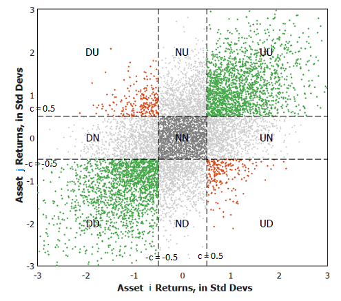
By introducing the Gerber threshold $c \in [0,1]$, this scatter plot can be partitioned into nine different subsets:

• The subset $UU$, containing the standardised joint returns for which both asset returns are above $c$
• The subset $DD$, containing the standardised joint returns for which both asset returns are below $-c$
• The subset $NN$, containing the standardised joint returns for which both asset returns are above $-c$ and below $c$
• …

The Gerber statistic $g_{i,j}$ is then defined as¹

\[g_{i,j} = \frac{n_{i,j}^{UU} + n_{i,j}^{DD} - n_{i,j}^{UD} -n_{i,j}^{DU}}{T - n_{i,j}^{NN}}\]

, where:

• $n_{i,j}^{UU}$ (resp. $n_{i,j}^{DD}$) is the number of standardised joint returns belonging to the subset $UU$ (resp. $DD$), which are termed concordant pairs of returns³ and are coloured in green in Figure 1
• $n_{i,j}^{UD}$ (resp. $n_{i,j}^{DU}$) is the number of standardised joint returns belonging to the subset $UD$ (resp. $DU$), which are termed discordant pairs of returns³ and are coloured in red in Figure 1
• $n_{i,j}^{NN}$ is the number of standardised joint returns belonging to the subset $NN$, which are considered as noise and are coloured in grey in Figure 1

Interpretation

The definition of the Gerber statistic makes it a measure of co-movement more robust to outliers and to noise than the
Pearson correlation coefficient.

Indeed, as highlighted in Gerber et al.¹:

• The Gerber statistic is insensitive to extreme[ly large or small] movements that distort [the Peason correlation coefficient]¹, because the magnitude of asset returns above or below the Gerber threshold $c$ is not taken into account
• The Gerber statistic is insentitive to small movements that may simply be noise¹, because a Gerber threshold of at least $c = 0.5$ is advocated in practice

From this perspective, the Gerber statistic is especially well suited for financial time series, which often exhibit extreme movements and a great amount of noise¹.

Alternative definitions

Flint and Polakow² reference three existing variations of the Gerber statistic and note that these alternative definitions materially change[] the resultant measure, to the point that the three GS variants in press should arguably be viewed as entirely separate dependence measures².

For the sake of clarity, this blog post will only discuss the variant termed the Gerber statistic in Gerber et al.¹.

Example of computation

Gerber et al.¹ illustrate the computation of the Gerber statistic using the $T = 24$ monthly returns⁴ of the asset pair S&P 500 (SPX) - Gold (XAU) over the period January 2019 - December 2020.

I propose to re-use the same example and to validate the computation thanks to the SPX - XAU returns available in the Google sheet associated to this post.

Figure 2 represents the scatter plot of the standardised joint returns of these two assets overlaid with the nine subsets corresponding to a Gerber threshold of 0.5.

Figure 2. Scatter plot of standardised joint returns of SPX - XAU partitioned into nine subsets by a Gerber threshold equal to 0.5, January 2019 - December 2020.

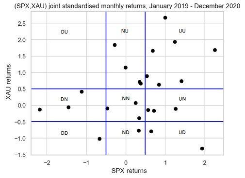
Figure 2 is exactly the same as the figure in panel A of exhibit A2 of Gerber et al.¹, so that the computation of the Gerber statistic should result in a value of ~0.286.

Let’s double check this.

From Figure 2, we have:

• $n_{SPX,XAU}^{UU} = 7$, $n_{SPX,XAU}^{DD} = 1$
• $n_{SPX,XAU}^{UD} = 0$, $n_{SPX,XAU}^{DU} = 2$
• $n_{SPX,XAU}^{NN} = 3$

So that:

\[g_{SPX,XAU} = \frac{7 + 1 - 0 - 2}{24 - 3} = \frac{2}{7} \approx 0.286\]

All good!

The Gerber correlation matrix

Let be:

• $n$, the number of assets in a universe of assets
• $r_{i,1},…,r_{i,T}$, the return of the asset $i=1..n$ over each time period $t=1..T$
• $c \in [0,1]$, the Gerber threshold

The asset Gerber correlation matrix $G \in \mathcal{M}(\mathbb{R}^{n \times n})$, also called the Gerber matrix, is then defined by:

\[G_{i,j} = g_{i,j}, i=1..n, j=1..n\]

, where $g_{i,j}$ is the Gerber statistic between asset $i$ and asset $j$.

The Gerber covariance matrix

Let be:

• $n$, the number of assets in a universe of assets
• $r_{i,1},…,r_{i,T}$, the return of the asset $i=1..n$ over each time period $t=1..T$
• $\sigma_1,…,\sigma_n$, the asset standard deviations (i.e., volatilities)
• $c \in [0,1]$, the Gerber threshold

The asset Gerber covariance matrix $\Sigma_G \in \mathcal{M}(\mathbb{R}^{n \times n})$ is then defined by:

\[\left( \Sigma_{G} \right)_{i,j} = g_{i,j} \, \sigma_i \, \sigma_j, i=1..n, j=1..n\]

, where $g_{i,j}$ is the Gerber statistic between asset $i$ and asset $j$.

Implementation in Portfolio Optimizer

Portfolio Optimizer implements two endpoints related to the Gerber statistic:

• /assets/correlation/matrix/gerber, to compute the Gerber correlation matrix
• /assets/covariance/matrix/gerber, to compute the Gerber covariance matrix

Empirical performances

Gerber et al.¹ analyze the empirical performance of the Gerber covariance matrix within the Markowitz’s mean-variance framework.

For this, they consider a universe of nine asset classes:

• US large cap stocks, represented by the S&P 500 index
• US small cap stocks, represented by the Russell 2000 index
• Developed markets ex. US and Canada large and mid cap stocks, represented by the MSCI EAFE index
• Emerging markets large and mid cap stocks, represented by the MSCI Emerging Markets index
• US treasuries, government-related and corporate bonds, represented by the Bloomberg Barclays US Aggregate Bond index
• US high yield corporate bonds, represented by the Bloomberg Barclays US Corporate High Yield Bond index
• US real estate, represented by the FTSE NAREIT all equity REITS index
• Gold
• Commodities, represented by the S&P GSCI Goldman Sachs Commodity index

, inside which they backtest the following portfolio investment strategy over the period January 1988 - December 2020:

1. At the end of each month, compute mean-variance input estimates over the past 24 months of returns
   • The average return vector $\mu = \left( \mu_{SPX},…,\mu_{SPGSCI} \right)$
   • The sample covariance matrix $\Sigma$
   • The Ledoit-Wolf shrunk covariance matrix $\Sigma_{LW}$⁵
   • The Gerber covariance matrix $\Sigma_{G}$
2. Then, compute no-short-sales constrained mean-variance efficient portfolios⁶ with an annualized volatility target of 3%, 5%, …, 15%
   • Using $\mu$ and $\Sigma$
   • Using $\mu$ and $\Sigma_{LW}$
   • Using $\mu$ and $\Sigma_{G}$

Figure 3, reproduced from Gerber et al.¹, illustrates the resulting three ex post mean-variance efficient frontiers in the case of a Gerber threshold equal to 0.5.

Figure 3. Nine-asset universe, ex post mean-variance efficient frontiers with a Gerber threshold equal to 0.5, January 1990 - December 2020. Source: Gerber et al.

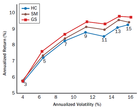
On this figure, it is pretty clear that the efficient frontier corresponding to the Gerber covariance matrix dominates the two other efficient frontiers⁷.

Based on these empirical findings, using the Gerber covariance matrix as an alternative to both [the sample covariance matrix] and to the shrinkage estimator of Ledoit and Wolf¹ seems really compelling.

Nevertheless, some practicalities must be discussed first.

Practical considerations

Robustness of the empirical study of Gerber et al.¹

In order to determine whether the empirical performances reported in Gerber et al.¹ are robust to slight changes in implementation details⁸, I propose to reproduce the backest of the portfolio investment strategy detailled in the previous section using Portfolio Optimizer⁹.

To be noted that because Portfolio Optimizer does not support Ledoit-Wolf type shrinkage at the date of publication of this post¹⁰, I am only able to compare the Gerber covariance matrix with the historical covariance matrix.

The two reproduced ex post mean-variance efficient frontiers are displayed in Figure 4 in the case of a Gerber threshold equal to 0.5.

Figure 4. Reproduced nine-asset universe, ex post mean-variance efficient frontiers with a Gerber threshold equal to 0.5, January 1990 - December 2020.

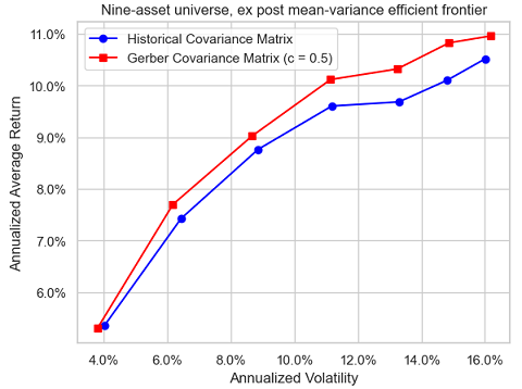
Figure 3 and Figure 4 are pretty close¹¹, except really for the mean-variance efficient portfolio with an annualized volatility target of 11%, which confirms the robustness in terms of reproducibility of the empirical study of Gerber et al.¹.

Influence of the Gerber threshold

The Gerber statistic, the Gerber correlation matrix and the Gerber covariance matrix all depend on the Gerber threshold, so that it is important to understand the impact of varying the Gerber threshold on these quantities.

In the case of two assets, this impact is extensively studied in Flint and Polakow² thanks to numerical simulations of joint normal and joint non-normal return distributions. Their conclusion is that the dependency of the Gerber statistic on the Gerber threshold is highly non trivial…

On my (less ambitious) side, I will study the impact of varying the Gerber threshold from 0 to 1 in increments of 0.1 on the backest of the portfolio investment strategy detailled in the previous section.

Figure 5 (resp. Figure 6) illustrates the evolution of the resulting portfolio investment strategy equity curves for an ex ante annualized volatility target of 5% (resp. 10%).

Figure 5. Reproduced nine-asset universe, influence of the Gerber threshold, ex ante annualized volatility target of 5%, January 1990 - December 2020.

Figure 6. Reproduced nine-asset universe, influence of the Gerber threshold, ex ante annualized volatility target of 10%, January 1990 - December 2020.

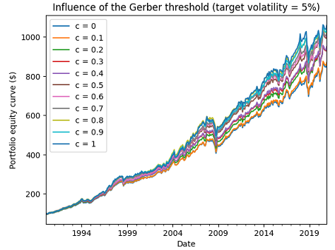
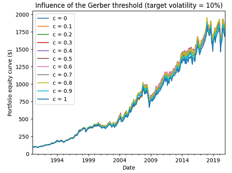
Figure 6 shows that the influence of the Gerber threshold on performances can be neglictible, which is very good news.

Unfortunately, Figure 5 shows on the contrary that the influence of the Gerber threshold on performances can be non-neglictible at all, which is bad news.

This leads to the question of how to “best” chose the Gerber threshold in practice.

How to choose the Gerber threshold?

From the definition of the Gerber statistic, the higher the Gerber threshold:

• The smaller the size of the “signal” subsets $UU$, $DD$, $UD$ and $DU$
• The greater the size of the “noise” subset $NN$

As a consequence, it would make sense to choose the Gerber threshold dynamically, as a function of the “signal-to-noise ratio” of the considered universe of assets.

In the context of the portfolio investment strategy detailled in the previous section, I experimented with a simple approach based on past risk-adjusted performances:

1. At the end of each month, compute mean-variance input estimates over the past 24 months of returns
   • The average return vector $\mu = \left( \mu_{SPX},…,\mu_{SPGSCI} \right)$
2. Then, for each annualized volatility target $v\%$
   • Compute the Gerber threshold $c^*$ which maximizes the Sharpe ratio of the associated portfolio investment strategy over the past 24 months¹² of returns
   • Compute the Gerber covariance matrix $\Sigma_{G^*}$ using the Gerber threshold $c^*$
   • Compute the no-short-sales constrained mean-variance efficient portfolio with an annualized volatility target of $v\%$, using $\mu$ and $\Sigma_{G^*}$

Figure 7 illustrates the evolution of the resulting portfolio investment strategy equity curve for an ex ante annualized volatility target of 5%.

Figure 7. Reproduced nine-asset universe, fixed v.s. adaptative Gerber threshold, ex ante annualized volatility target of 5%, January 1992 - December 2020.

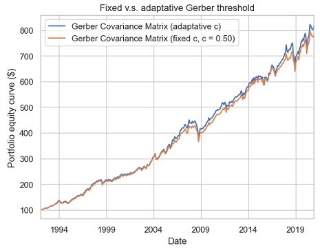
From Figure 7, it appears that this simple data-driven method to choose the Gerber threshold is able to match the performances of the best Gerber threshold chosen in hindsight¹³ ($c = 0.5$).

Some (annualized) statistics to support this observation:

	Gerber portfolio (fixed c = 0.50)	Gerber portfolio (adaptative c)
Average return	7.6%	7.9%
Volatility	6.2%	6.2%
Sharpe ratio	1.26	1.23

Of course, no generic conclusion can be drawn from this example, but I do think that the adaptative computation of the Gerber threshold would be an interesting research topic.

Positive semidefinitess of the Gerber correlation matrix

Gerber et al.¹ mention that

In the empirical studies performed, and for all cases of Gerber thresholds $c$ considered, we always observe the […] Gerber matrix G to be positive semidefinite

, but give no formal proof that the Gerber correlation matrix is positive semidefinite in general.

It is thus natural to wonder whether this is the case, all the more because positive semidefinitess is usually lacking in other correlation matrices built from robust pairwise scatter estimates¹⁴¹⁵.

Hopefully, the Gerber correlation matrix is indeed positive semidefinite, as established in the paper Proofs that the Gerber Statistic is Positive Semidefinite from Gerber et al.¹⁶

Note:

• The initial version of this post stated that there were no proof that the Gerber correlation matrix was a positive semidefinite matrix; this was incorrect, as a proof was available on Mr Enrst website.

Usage of the Gerber statistic beyond mean-variance

In their paper, Gerber et al.¹ confine [their] analysis to the mean–variance optimization (MVO) framework of Markowitz.

What about other portfolio allocation frameworks, though?

Would the Gerber statistic be somewhat taylored to the mean-variance framework, for example because of a hidden relationship with quadratic utility?

To answer this question, I propose to adapt the portfolio investment strategy detailled inthe previous section to the risk parity framework, and more precisely to the equal risk contributions framework¹⁷, as follows:

1. At the end of each month, compute risk parity input estimates over the past 24 months of returns
   • The sample covariance matrix $\Sigma$
   • The Gerber covariance matrix $\Sigma_{G}$
2. Then, compute the no-short-sales constrained equal risk contributions portfolio
   • Using $\Sigma$
   • Using $\Sigma_{G}$

Figure 8 illustrates the resulting portfolio investment strategy equity curves in the case of a Gerber threshold equal to 0.5.

Figure 8. Reproduced nine-asset universe, equal risk contributions with a Gerber threshold equal to 0.5, January 1990 - December 2020.

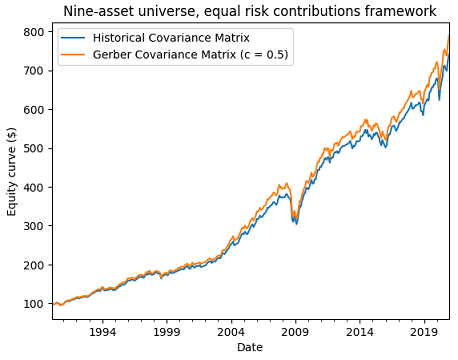
Figure 8 also empirically confirms that the Gerber covariance matrix also behaves properly in a non mean–variance framework.

Caveats

Non-uniform domination of the Gerber covariance matrix

Figure 3 and Figure 4 might give the wrong impression that the Gerber covariance matrix always dominates the sample covariance matrix in terms of ex post risk-return within the Markowitz’s mean-variance framework¹⁸.

In order to illustrate that this is not the case, I will backtest the same portfolio investment strategy as detailled in one of the previous sections, but this time with the ten-asset universe of the Adaptative Asset Allocation strategy¹⁹²⁰ from ReSolve Asset Management:

• U.S. stocks (SPY ETF)
• European stocks (EZU ETF)
• Japanese stocks (EWJ ETF)
• Emerging markets stocks (EEM ETF)
• U.S. REITs (VNQ ETF)
• International REITs (RWX ETF)
• U.S. 7-10 year Treasuries (IEF ETF)
• U.S. 20+ year Treasuries (TLT ETF)
• Commodities (DBC ETF)
• Gold (GLD ETF)a universe of nine asset classes:

This universe is very similar to the nine-asset universe used in Gerber et al.¹, because it is also well-diversified in terms of asset classes.

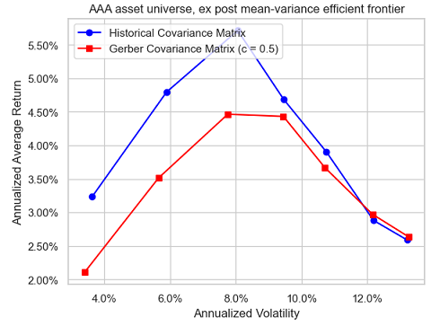
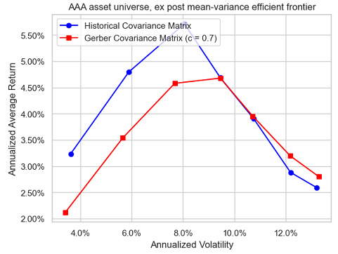
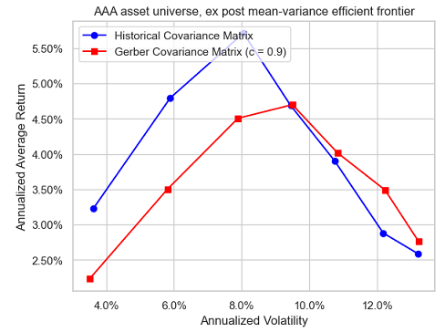
Unfortunately, with this universe, the ex post efficient frontier corresponding to the Gerber covariance matrix does not always dominate anymore the ex post efficient frontier corresponding to the sample covariance matrix, as can be seen in Figure 9, Figure 10 and Figure 11.

Figure 9. AAA universe, ex post mean-variance efficient frontiers with a Gerber threshold equal to 0.5, January 2007 - April 2023.

Figure 10. AAA universe, ex post mean-variance efficient frontiers with a Gerber threshold equal to 0.7, January 2007 - April 2023.

Figure 11. AAA universe, ex post mean-variance efficient frontiers with a Gerber threshold equal to 0.9, January 2007 - April 2023.

Influence of the number of observations

Because of its definition, the Gerber statistic must intuitively be more sensitive than the sample covariance matrix to measurement error²¹.

Still, in my own testing, I did not notice any excessive sensitivity²².

For example, Figure 12 is the equivalent of Figure 9 when daily asset returns are used instead of monthly returns.

Figure 12. AAA universe, ex post mean-variance efficient frontiers with a Gerber threshold equal to 0.5, January 2007 - April 2023, daily returns.

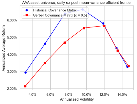
Comparing these two figures, it is hard to conclude that the Gerber covariance matrix is dramatically more sensitive to the number of observations than the sample covariance matrix²³.

That being said, Flint and Polakow² investigate the sensitivity of the Gerber statistic to estimation error more rigourously, and do find that there is considerable variation in the GS when estimated with limited observations².

So, better to err on the side of caution here.

Conclusion

I hope that thanks to this post you now have a good overview of the Gerber statistic, along with some of the practical concerns associated with its usage.

As Flint and Polakow² put it:

Overall, the GS is an interesting conditional dependence metric, but not without its flaws or caveats.

If you have any questions, or if you would like to discuss further, feel free to connect with me on LinkedIn or to follow me on Twitter.

–

1. See Gerber, S., B. Javid, H. Markowitz, P. Sargen, and D. Starer (2022). The gerber statistic: A robust co-movement measure for portfolio optimization. The Journal of Portfolio Management 48(2), 87–102. ↩ ↩² ↩³ ↩⁴ ↩⁵ ↩⁶ ↩⁷ ↩⁸ ↩⁹ ↩¹⁰ ↩¹¹ ↩¹² ↩¹³ ↩¹⁴ ↩¹⁵ ↩¹⁶ ↩¹⁷ ↩¹⁸ ↩¹⁹

2. See Flint, Emlyn and Polakow, Daniel A., Deconstructing the Gerber Statistic. ↩ ↩² ↩³ ↩⁴ ↩⁵ ↩⁶ ↩⁷

3. More precisely, Gerber et al.¹ define a concordant pair of returns as a pair which both components pierce their thresholds while moving in the same direction and a discordant pair of returns as a pair whose components pierce their thresholds while moving in opposite directions. ↩ ↩²

4. All asset returns considered in this blog post are total returns. ↩

5. See Ledoit, O., and M. Wolf. 2004. “Honey, I Shrunk the Sample Covariance Matrix.” The Journal of Portfolio Management 30 (4): 110–119. ↩

6. The exact implementation details used by Gerber et al.¹ can be found in the Python code associated to their paper; one important detail to note is that when there is no mean-variance efficient portfolio with the desired volatility, the minimum variance portfolio or the maximum return portfolio is used instead. ↩

7. The same conclusion applies for the two other values of the Gerber threshold, c.f. Gerber et al.¹. ↩

8. In particular, when there is no mean-variance efficient portfolio with a desired volatility because the desired volatility is too low, it might be more in line with the mean-variance framework to use a partially invested portfolio v.s. the minimum variance portfolio as in Gerber et al.¹. ↩

9. I would like to thank Mr William Smyth²⁴ for providing me returns data for the nine-asset universe. ↩

10. It’s definitely on the to do list, though. ↩

11. In addition to the difference in managing the portfolio volatility constraint⁸, there are other subtle differences in my reproduction of the backtest of Gerber et al.¹; for example, I do not consider any transaction cost, I use the arithmetic average return of indexes and not their geometric average return, etc. ↩

12. The performances of the method seem to be robust w.r.t. the lookback period; to be noted that a lookback period of 12 months results in the best performances, but I chose 24 months to be consistent with the lookback period used to compute mean-variance input estimates. ↩

13. In terms of the Sharpe ratio of the resulting portfolio investment strategy, the best Gerber threshold among the thresholds displayed in Figure 5 is equal to 0.5. ↩

14. Zhao, Tuo, et al. Positive Semidefinite Rank-Based Correlation Matrix Estimation With Application to Semiparametric Graph Estimation. Journal of Computational and Graphical Statistics, vol. 23, no. 4, 2014, pp. 895–922. JSTOR ↩

15. See F.A. Alqallaf, K.P. Konis, R.D. Martin, and R.H. Zamar. Scalable robust covariance and correlation estimates for data mining. In Proceedings of the Eighth ACM SIGKDD International Conference on Knowledge Discovery and Data Mining, pages 14-23. ACM, 2002. ↩

16. See S. Gerber, H. Markowitz, P. Ernst, Y. Miao, B. Javid, P. Sargen, Proofs that the Gerber Statistic is Positive Semidefinite, arXiv. ↩

17. See Richard, Jean-Charles and Roncalli, Thierry, Constrained Risk Budgeting Portfolios: Theory, Algorithms, Applications & Puzzles. ↩

18. Which, to be clear, is not at all the conclusion of Gerber et al.¹. ↩

19. See Butler, Adam and Philbrick, Mike and Gordillo, Rodrigo and Varadi, David, Adaptive Asset Allocation: A Primer. ↩

20. The associated returns data have been retrieved using Tiingo. ↩

21. In this context, the measurement error is due to the short length of the time series of asset returns that are typically used for covariance matrix estimation. ↩

22. To be noted that I only used the Gerber statistic with well diversified universes of assets and not with let’s say a universe of stocks (S&P 500…). ↩

23. Or at the very least, if it really is, this does not translate into dramatically different risk-return performances, which is what ultimately matters from a portfolio management perspective. ↩

24. See William Smyth, Daniel Broby, An enhanced Gerber statistic for portfolio optimization, Finance Research Letters, Volume 49, 2022, 103229. ↩