The Log-Linear Regression: Usage for Long-Term Financial Asset Analysis

In finance, various studies have explored the use of regression models in forecasting stock prices […] based on historical data and other relevant variables¹.

Among these models, the log-linear regression model is of particular importance due to its relationship with the geometric Brownian motion (GBM) asset pricing model introduced by Paul Samuelson² and at the heart of the Black–Scholes formula³.

In this blog post, I will describe that regression model, explain why it is theoretically relevant for analyzing the evolution of asset prices over the long-term and show how it can be used in practice to estimate an asset’s relative valuation based on its historical price levels.

As a side note, analyzing assets through a log-linear regression model is part of what proposes the Hiboo financial analysis platform through what they call the hiboo regression line⁴.

Mathematical preliminaries

Below is an extract of Samuelson².

Let the price of an asset be defined for all time and be denoted by $S_t$.

If we stand at the time $t$, we know with certainty $S_t$ and all of its past values $S_{t-T}, T=1..t$.

Its future price $S_{t+T}, T=1..$, though, is knowable only in some probability sense, its probability distribution being in the most general case a function of the whole past profile of $S_{t-T}, T=1..t$.

Over the years, many different types of models have been suggested for the modelling of [that probability distribution], some more complicated than others⁵.

The least ambitious goal, which has received a lot of attention since the beginning of this century starting with Bachelier⁶, is to give a statistical/mathematical model which is capable of describing the behavior of a single stock via one stochastic process⁵.

Samuelson’s pricing model² is such a statistical model, under which the asset price is assumed to follow a geometric Brownian motion process:

\[d S_t = \mu S_t dt + \sigma S_t dW_t\]

, where:

• $\mu$ is the (constant) continuously-compounded expected return of the stochastic process, also called the log-drift
• $\sigma$ is the (constant) volatility of the stochastic process
• $W_t$ is a standard Brownian motion with $ W_t \sim \mathcal{N} \left( 0, t \right) $

As a consequence⁷, the log-price process $\log S_t $ follows a $\sigma$-scaled Brownian motion with drift $\mu - \frac{1}{2} \sigma^2$ and starting at $\log S_0$:

\[\log S_t = \log S_0 + \left( \mu - \frac{1}{2} \sigma^2 \right) t + \sigma W_t\]

In other words, at any time $t$, the asset price $S_t$ follows a log-normal probability distribution:

\[\log S_t \sim \mathcal{N} \left( \log S_0 + \left( \mu - \frac{1}{2} \sigma^2 \right) t, \sigma^2 t \right)\]

As another consequence, at any time $t$, the asset log-return $ \log \frac{S_t}{S_{t-1}} $ follows a normal distribution:

\[\log \frac{S_t}{S_{t-1}} \sim \mathcal{N} \left( \mu - \frac{1}{2} \sigma^2, \sigma^2 \right)\]

Log-linear regression for asset prices

Log-linear regression

Let’s consider the textbook bivariate linear regression model relating a dependent variable $Y$ to an independent variable $X$:

\[Y = \alpha + \beta X + \varepsilon\]

, where:

• $\alpha$ is the intercept of the linear regression line
• $\beta$ is the slope of the linear regression line
• $\varepsilon$ is the error term, representing the unexplained variation in $Y$

Under certain circumstances, a logarithmic transformation⁸ can be applied to either or both variables, for example when modelling exponential growth or power-law relationships.

When the dependent variable is log-transformed while the independent variable remains in its original scale, the resulting model is called a log-linear regression model:

\[\log Y = \alpha + \beta X + \varepsilon\]

Log-linear regression applied to idealized asset prices

Let’s consider an asset whose price $S_t$ follows a geometric Brownian motion, with observed prices $S_0,S_1,…,S_{T}$ at times $t=0,1,…,T$.

Applying the log-linear regression described in the previous sub-section to these asset prices gives:

\[\log S_t = \hat{\alpha}_T + \hat{\beta}_T t + \hat{\varepsilon}_t, \qquad t=0,...,T\]

Now, because the asset log-prices satisfie the relationship:

\[\log S_t = \log S_0 + \left( \mu - \frac{1}{2} \sigma^2 \right) t + \sigma W_t\]

, and by comparing the two equations, the log-linear regression estimates the following two parameters:

• $\hat{\alpha}_T$, the log-linear regression intercept, which is an estimate of the initial asset log-price $\log S_0$.
• $\hat{\beta}_T$, the log-linear regression slope, which is an estimate of the asset log-price drift $ \mu - \frac{1}{2}\sigma^2 $.

The log-linear regression thus provides a direct estimate of the asset’s long-term continuously compounded growth rate.

As an illustration, Figure 1 depicts 10,001 simulated price observations over 100 years of an asset whose prices follow a geometric Brownian motion⁹ together with its estimated log-linear regression line.

Figure 1. Example of asset whose simulated prices follow a geometric Brownian motion, plus estimated log-linear regression line.

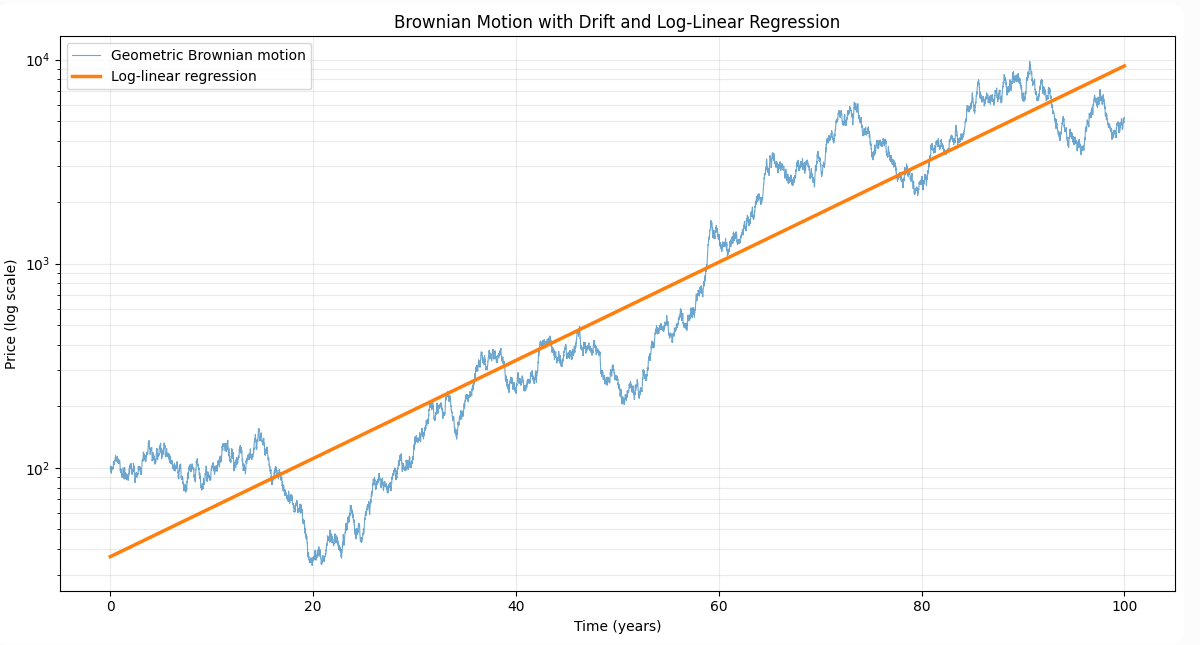
From Figure 1, it appears that despite their short-term fluctuations, simulated asset prices tend to follow - in a loose sense - the estimated log-linear regression line over the long term.

This is actually a general result.

Indeed:

• The strong law of large numbers for the Brownian motion allows to establish that $ \hat{\beta}_T \xrightarrow[T\to\infty]{\text{a.s.}} \mu-\frac{1}{2}\sigma^2 $.

  In other words, as the observation horizon increases, the estimated log-linear regression slope converges almost surely to the true asset log-price drift.

• With $D_t = S_t - \left( \log S_0 + \left( \mu-\frac{1}{2}\sigma^2 \right) t \right)$ the log-price deviation, $D_t = \sigma W_t$ and the strong law of large numbers for the Brownian motion implies that $ \frac{D_t}{t} \longrightarrow 0$ almost surely.

  Here, as the observation horizon increases, deviations of the asset log-price from its log-price trend line become negligible almost surely.

Both results stitched together imply that over the long term, deviations of the asset log-price from the estimated log-linear regression line become negligible¹⁰.

Beyond the asset’s long-term growth rate, the log-linear regression also enables to (indirectly) estimate the asset volatility.

Mathematically, this is done by computing the standard error¹¹ $s_e$ of the log-linear regression defined by

\[s_e = \sqrt{\frac{1}{T-1} \sum_{i=0}^{T} \left(\log S_i-\hat \alpha_T -\hat\beta_T i\right)^2}\]

and using it to compute standard deviation bands $\pm k s_e, k=1,2…$.

These bands, popularized in technical analysis by Andersen¹², allow to visualize historical price fluctuations around the estimated log-linear regression line and have the interesting property that a higher (resp. lower) asset volatility $\sigma$ leads to wider (resp. narrower) bands around that line.

This is because the expected distance on the log-price scale between the estimated log-linear regression line and the $\pm 1$ standard deviation bands sastisfy $ \sqrt{ \mathbb E[s_e^2] } = \sigma \sqrt{ \frac{T+2}{6}} $.

Figure 2 depicts another set of 10,001 simulated price observations over 100 years of an asset whose price follows a geometric Brownian motion⁹, this time together with both the associated estimated log-linear regression line and the $\pm 1$ and $\pm 2$ standard deviation bands.

Figure 2. Example of asset whose simulated price follows a geometric Brownian motion, plus associated estimated log-linear regression line and standard deviation bands.

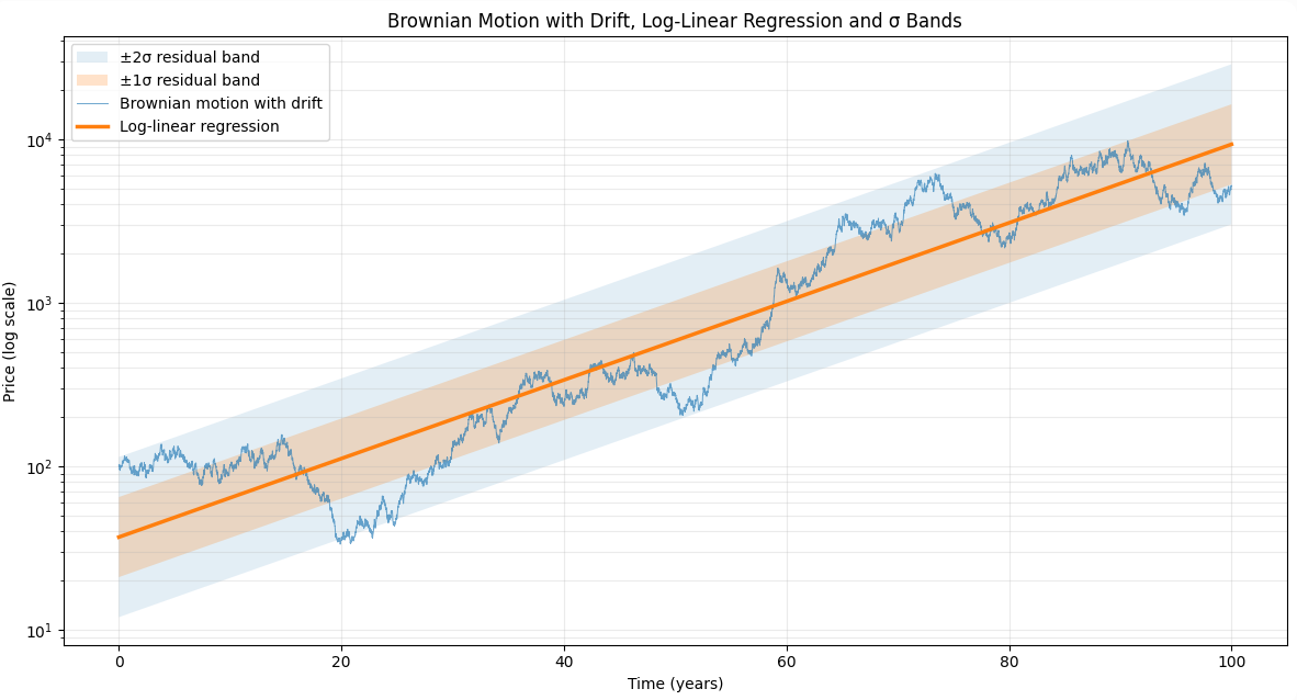
The visual representation depicted in Figure 2 is sometimes called a logarithmic regression channel in technical analysis.

As a side note, the primary usage for these standard deviation bands in practice is usually to identify prices that are unusually high or low relative to the estimated log-linear regression line.

Nevertheless, one must be careful with that usage, because these bands offer no specific probabilistic coverage properties under a geometric Brownian motion model and in particular, they are not mean-reverting bands¹³.

What can be said, though, is that prices cannot remain permanently inside any of these bands and must cross the estimated log-linear regression line¹⁴ infinitely often, in both directions¹⁵.

This is a consequence of the Brownian motion property that $\limsup_{t\to\infty} D_t=+\infty$ and $\liminf_{t\to\infty}D_t=-\infty$ almost surely.

But here, we are talking about the (mathematical) long-term; in terms of immediate future, there is no finite time by which a crossing is actually guaranteed…

Log-linear regression applied to real asset prices

Let’s immediately address the elephant in the room: in practice, it is very well know that (unconditional) asset log-returns do not follow a Gaussian distribution, so that in particular asset prices cannot follow a geometric geometric Brownian motion⁵.

Nevertheless, it has been observed that as one increases the time scale over which returns are calculated, their distribution looks more and more like a normal distribution¹⁶.

This stylized fact of financial asset returns - called aggregational gaussianity - is illustrated in Figure 3.

Figure 3. Empirical densities of the IBM log-returns v.s. estimated normal density, 2th January 1973 - 25th January 1996. Source: Rydberg.

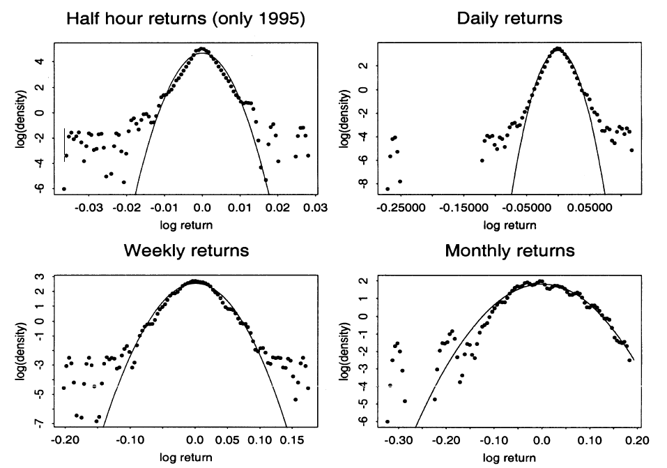
Theoretically, this stylized fact is supported by the result that for decreasing sampling frequencies the central limit law sets in and the distribution of the log returns tends towards a Gaussian law⁵, with decreasing sampling frequencies […] equivalent to aggregation⁵ when working with log-returns.

So, depending on the observation frequency (monthly, quarterly, yearly…) and with a couple of additional assumptions (constant variance…), a geometric Brownian motion model for real asset prices might be good enough, especially since the intended purpose of using the log-linear regression would be long-term asset prices analysis.

That being mentioned, imposing these additional assumptions comes with other issues.

A pragmatic way out of this mess is to assume that asset prices follow a time-inhomogeneous geometric Brownian motion, with time-varying log-drift $\mu_t$ and volatility $\sigma_t$ parameters.

Then, depending on the situtation at hand (stock with stable business characteristics such as a mature company, stock suffering from a structural change like banks after 2008…), these time-varying parameters can be assumed to be:

• Slowly varying, which allows log-linear regression to be used to study the asset over a long period¹⁷.
• Subject to structural breaks, which prevent a single log-linear regression over the entire historical period from being used but which still allows log-linear regression to be used to study the asset over individual periods between breaks¹⁸.
• Following other dynamics, which requires a more detailed analysis or a different modelling approach altogether.

The first situation is obviously the best one, as mentioned by Hiboo in one of their videos detailing a checklist for finding stocks “compatible” with long-term log-linear regression analysis.

For convenience, that checklist is summarized in Figure 4.

Figure 4. Hiboos's checklist for applying log-linear regression to an individual stock. Source: Hiboo.

As a final point of attention when applying log-linear regression for decision making, it must be highlighted that the estimated log-linear regression line and standard deviation bands are computed over the past periods $0,1,…,T$ using all the available asset prices $S_0,S_1,…,S_{T}$.

By construction, the estimated log-linear regression line at time $t=i$ with $0 \leq i \leq T$ thus uses future asset prices $S_{i+1},…,S_{T}$, which is a textbook case of data leakage.

It is important to keep this in mind when visually interpreting graphs like the one displayed in Figure 2, which might otherwise give a false impression of confidence.

It is also important to keep this in mind when performing backtests on trading strategies that rely on log-linear regression, because this data leakage basically invalidates them…

Hopefully, the solution to this problem is well-known and simply consists in using asset prices up to time $t=i$ when estimating the log-linear regression line and standard deviation bands over the past periods $0,1,…,i$, which is called recursive least squares (RLS) estimation as opposed to ordinary least squares (OLS) estimation.

More on this later.

Implementation in Portfolio Optimizer

Portfolio Optimizer provides the endpoint /assets/prices/logarithmic-regression-channel that allows to easily compute log-linear regression on asset prices.

This endpoint supports several methods of estimation for the log-linear regression line and standard deviation bands:

• Ordinary least squares (data leakage)
• Robust least squares (data leakage)
• Recursive least squares (no data leakage)

Example of usages

Analyzing the long-term behaviour of individual stocks

As a first example of usage, I propose to illustrate the behaviour of log-linear regression as a support for trading decisions on individual stocks.

For this, I will take two examples:

• Air Liquide, a “boring” individual stock satisfying all the conditions listed in Figure 4
• Viridien, a very volatile individual stock subject to major structural changes

Air Liquide

Figure 5 depicts the log-linear regression line and standard deviation bands as estimated by Hiboo for the Air Liquide stock using adjusted close prices over the period 3rd January 1992 to 12th October 2026.

Figure 5. Hiboos's estimated log-linear regression line and standard deviation bands, Air Liquide, 3rd January 1992 - 12th October 2026. Source: Hiboo.

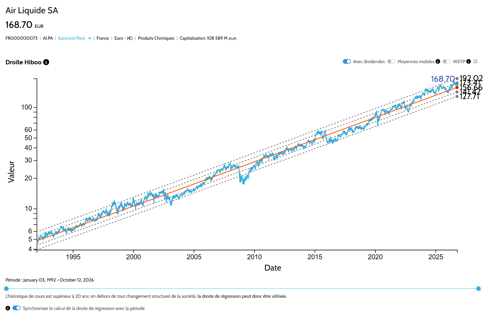
For comparison, Figure 6 depicts the log-linear regression line and standard deviation bands as estimated by Portfolio Optimizer using similar prices.

Figure 6. Portfolio Optimizer's estimated log-linear regression line and standard deviation bands, Air Liquide, 3rd January 1992 - 12th October 2026.

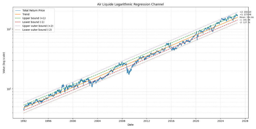
From Figure 5 and Figure 6¹⁹, it is clearly visible that the Air Liquide stock price exhibits a very stable behaviour over the past ~35 years, which supports for example the idea to project its estimated log-linear regression line over a future time period so as to guesstimate potential future stock prices.

Yet, as mentioned in a previous section, that stable behaviour is potentially an illusion due to the way the log-linear regression line is estimated.

To find out for sure, Figure 7 is the same as Figure 6 except that recursive least squares have been used to estimate the log-linear regression line and standard deviation bands instead of ordinary least squares.

Figure 7. Portfolio Optimizer's estimated log-linear regression line and standard deviation bands using recursive least squares, Air Liquide, 3rd January 1992 - 12th October 2026.

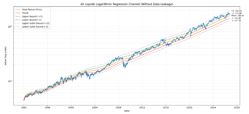
On Figure 7, the very stable behaviour of Figure 6 is definitely still present, which empirically validates the log-linear regression approach to analyzing the Air Liquide stock.

Those two figures are not identical, though, with for example:

• Just before the COVID-19 outbreak, Air Liquide stock price around its +1 standard deviation band in Figure 6 v.s. around its +2 standard deviation band in Figure 7
• Just after the COVID-19 outbreak, Air Liquide stock price around its -2 standard deviation band in Figure 6 v.s. around its -1 standard deviation band in Figure 7

As it turns out, the standard regression bands computed without any data leakage can be used to create a mean-reversion²⁰ trading strategy that can easily be backtested:

• Buy the Air Liquide stock when it is becomes relatively cheap (= log-price below its -1 standard deviation band)
• Sell the Air Liquide stock when it becomes relatively expansive (= log-price above its +2 standard deviation band)

Figure 8 compares that trading strategy to buy and hold.

Figure 8. Mean-reversion trading strategy based on estimated log-linear regression standard deviation bands v.s. buy and hold, Air Liquide, 3rd January 1992 - 12th October 2026.

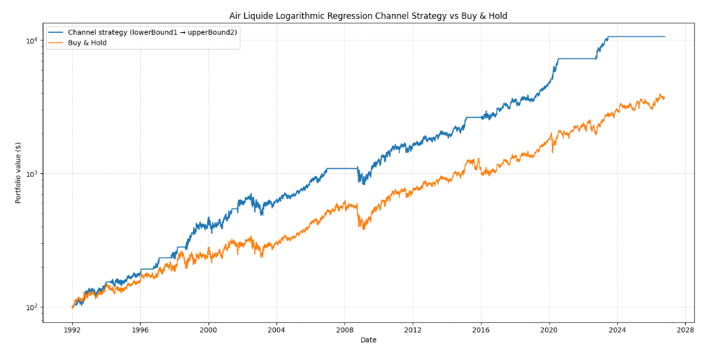
Main figures below.

Trading Strategy	CAGR	Annualized Sharpe Ratio (0)	Maximum (Daily) Drawdown
Mean-reversion trading strategy	14.36%	0.753	31.57%
Buy and hold	10.94%	0.547	39.43%

So, on this particular stock, a trading strategy based on the log-linear regression outperforms buy and hold by ~3.50% per year with less risk.

Viridien

Let’s now apply the same approach as in the previous sub-section to a very different individual stock.

Figure 9 depicts the log-linear regression line and standard deviation bands as estimated by Hiboo for the Viridien stock using adjusted close prices over the period 3rd January 1992 to 12th October 2026.

Figure 9. Hiboos's estimated log-linear regression line and standard deviation bands, Viridien, 3rd January 1992 - 12th October 2026. Source: Hiboo.

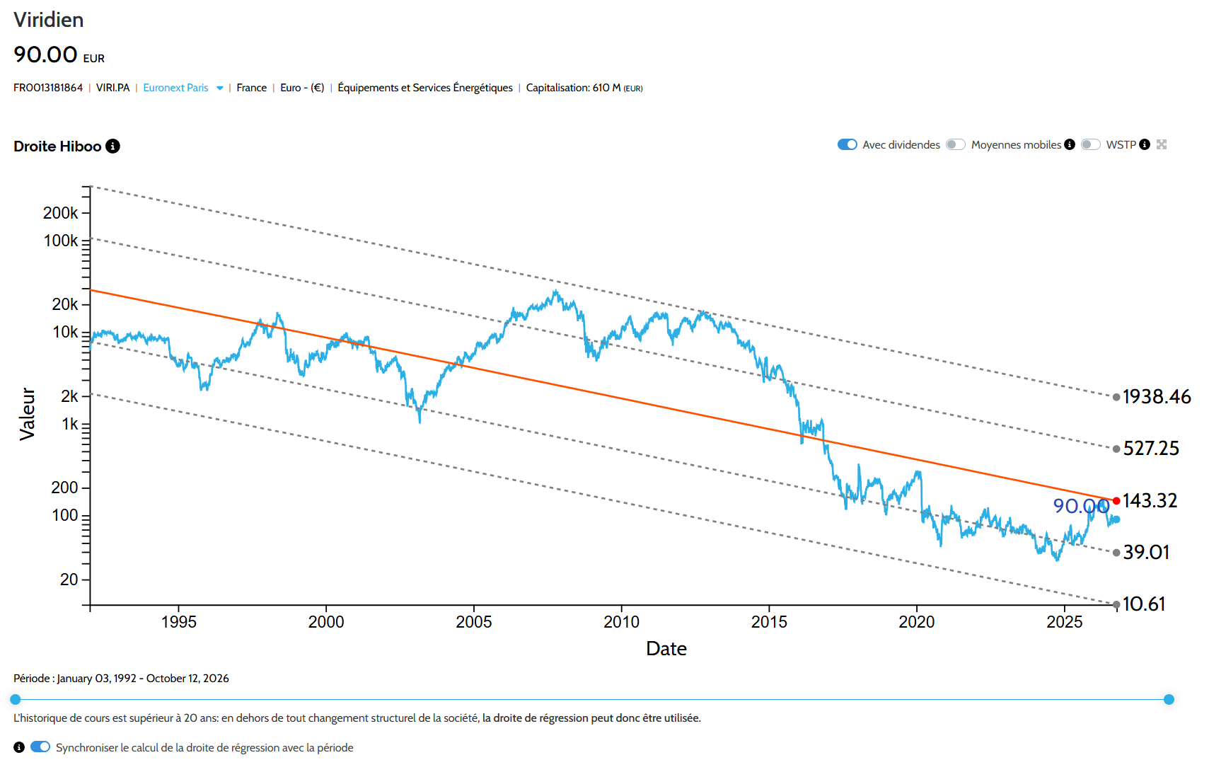
Figure 10 depicts the log-linear regression line and standard deviation bands as estimated by Portfolio Optimizer using recursive least squares and similar prices.

Figure 10. Portfolio Optimizer's estimated log-linear regression line and standard deviation bands using recursive least squares, Viridien, 3rd January 1992 - 12th October 2026.

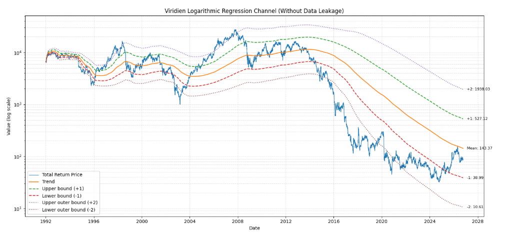
Contrary to Figure 5 and Figure 7, Figure 9 and Figure 10 are this time completely different in terms of estimated log-linear regression line and standard deviation bands!

In particular, the clear log-price downtrend in Figure 9 is not present anymore in Figure 10 and is replaced by a log-price trend break starting around 2016.

This situation illustrates the huge impact that data leakage can have on the analysis of the past behaviour of a stock and why - at the very least - ordinary least squares estimation should always be compared to recursive least squares estimation.

Figure 11 now compares the mean-reversion trading strategy to buy and hold in the case of Viridien.

Figure 11. Mean-reversion trading strategy based on estimated log-linear regression standard deviation bands v.s. buy and hold, Viridien, 3rd January 1992 - 12th October 2026.

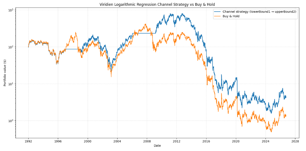
Main figures below.

Trading Strategy	CAGR	Annualized Sharpe Ratio (0)	Maximum (Daily) Drawdown
Mean-reversion trading strategy	-8.58%	0.087	-99.80%
Buy and hold	-11.60%	0.063	-99.88%

Thus, a trading strategy based on the log-linear regression again outperforms buy and hold by ~3.00% per year with less risk.

Unfortunately, that trading strategy alone²¹ is not sufficient to transform a losing stock into a winning stock, hence the importance of checklists like Hiboos’s in Figure 4.

Conclusion

Since Air Liquide and Viridien are nearly opposites in terms of stock price behaviour, the tests performed in the previous sub-sections give some confidence that using log-linear regression analysis as a support for trading decisions on individual stocks might be empirically justified.

Naturally, more tests would be needed to reach a definitive conclusion, but such an activity is out of scope of this blog post.

Analyzing the long-term behaviour of asset classes

Beyond individual stocks, log-linear regression analysis can also be performed on asset classes (equities, bonds, commodities…).

On a personal note, I think it even makes more sense, because:

• Asset classes typically²² do not go bust
• Asset classes might undergo structural changes, but such changes are typically well-identified and of macro nature like the 1973 structural change of the gold market
• Asset classes have longer price histories than individual assets

As an example, Figure 12 depicts the monthly evolution of the U.S. stock market over the period January 1871 - October 2026²³ in real terms, together with its RLS estimated log-linear regression line and standard deviation bands.

Figure 12. Portfolio Optimizer's estimated log-linear regression line and standard deviation bands using recursive least squares, Shiller's inflation-adjusted S&P Composite, January 1871 - October 2026.

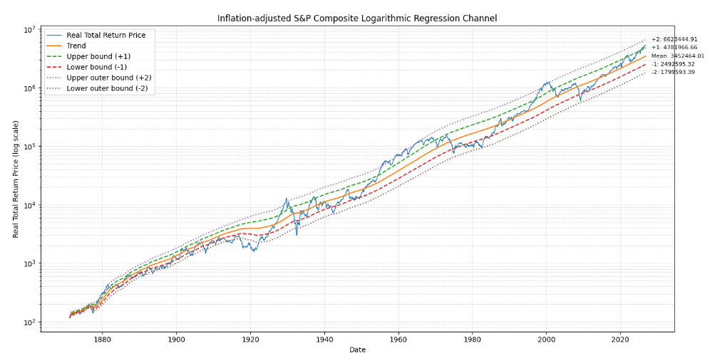
Thanks to Figure 12, it is possible to conclude that the U.S. stock market:

• Seems to follow a clean long-term log-price uptrend, especially since 1960
• Seems to be currently slightly overvalued compared to its long-term history (current prices around the +1 standard deviation band) but not in a comparable situation to let’s say the dot-com bubble (prices around +2 standard deviation band); of course, this does not rule out a vicious market crash, c.f. 1973 or 2022, but helps in contextualizing the “AI bubble”.

As a side note, and especially for long-term analysis like this over more than one century, dividends must absolutely be integrated into the prices of the asset under study, unlike what is sometimes done did.

Conclusion

This blog post presented the statistical framework of log-linear regression and its possible usage for the long-term analysis of asset prices.

By definiton, such a regression is a polynomial regression of order 1²⁴.

An interesting next step would be to investigate whether regressions of higher orders (2 - quadratic regression, 3 - cubic regression…) would result in better performances, for exemple in terms of associated trading strategies.

This is exactly the subject of the paper Polynomial Moving Regression Band Stocks Trading System by Cohen¹, to which the interested reader is referred.

To discover more uncommon subjects, feel free to connect with me on LinkedIn or follow me on Twitter.

–

1. See Gil Cohen, Polynomial Moving Regression Band Stocks Trading System, Risks 12: 166, 2024. ↩ ↩²

2. See Samuelson, P.A. (1965). Rational theory of warrant pricing. Industrial Management Review, 6(2), 13–39. ↩ ↩² ↩³

3. See Black, F and Scholes, M. (1973). The Pricing of Options and Corporate Liabilities. Journal of Political Economy, 81, 637-654. ↩

4. En français dans le texte, la droite hiboo. ↩

5. See Rydberg, Tina Hviid. “Realistic Statistical Modelling of Financial Data.” International Statistical Review / Revue Internationale de Statistique, vol. 68, no. 3, 2000, pp. 233–58. ↩ ↩² ↩³ ↩⁴ ↩⁵

6. See Bachelier, L. (1900, 1966). Theory de la Speculation, Gauthier-Villars, Paris, in The Random Character of Stock Market Prices, P. Cootner, ed, MIT Press, Cambridge. ↩

7. All these results are standard results related to the Brownian motion, and can be found in any textbook on stochastic processes. ↩

8. The natural logarithm. ↩

9. The geometric Brownian motion has an initial price of 100, an annual drift of 8% and an annual volatility of 20%. ↩ ↩²

10. Almost surely. ↩

11. The standard error of the log-regression represents the average distance that the observed [log] values fall from the [log] regression line²⁵. ↩

12. See Jon Andersen, Standard Error Bands, Traders issue: Stocks & Commodities V. 14:9 (375-379). ↩

13. The Brownian motion has no mean-reverting mechanism. ↩

14. More precisely, the true asset log-price trend, which - given enough data - is the same as the estimated log-linear regression line for all practical purposes. ↩

15. This is the mathematical translation of “cheap stocks can stay cheap for a long time” and “expansive stocks can stay expansive for a long time”… ↩

16. See R. Cont (2001) Empirical properties of asset returns: stylized facts and statistical issues, Quantitative Finance, 1:2, 223-236. ↩

17. Provided that the changes remain gradual enough for a single trend to remain meaningful. ↩

18. In particular, all data before the latest break needs to be discarded from the log-linear regression; for example, for banks, it means not taking into account stock prices from the banking sector before the new normal post-2008. ↩

19. Which are a near perfect match. ↩

20. As mentioned in this blog post, real asset prices do not follow a geometric Brownian motion process in practice, so that they can perfectly be mean-reverting. ↩

21. For this, other indicators should be used, like time series momentum indicators. ↩

22. Subject to discussion (world wars, countries defaulting on their debt…). ↩

23. Using total return data corrected for inflation available on Robert J. Shiller’s website. ↩

24. In log-prices. ↩

25. See Jim Frost, Standard error of the regression. ↩