Residualization of Risk Factors: Examples and Pitfalls
The most common approach to measuring portfolio (risk) factor exposures is linear regression analysis, which describes the relationship between a dependent variable - portfolio returns - and explanatory variables - factors - as linear.
One of the outputs of this analysis are the partial regression coefficients, also known as the betas ($\beta$). Each one of them measures the expected change in the portfolio returns associated with a change in one factor, holding all the other factors constant.
Problem is, factors are often correlated with one another in finance, so that holding all the other factors constant is not a realistic working assumption!
For example, in the Fama–French RM-RF, SMB and HML three-factor model original paper1, the correlation between the factors RM-RF and SMB is 0.32 and the correlation between the factors RM-RF and HML is -0.38.
When such correlations exist, a change in one factor will actually spill over into all the other correlated factors,
making the textbook interpretation of the beta coefficients difficult to use in practice2.
One possibility to solve this multicollinearity issue3, especially when there is only one problematic factor, is to use a mathematical trick called residualization.
This post will illustrate possible usages of residualization, using Portfolio Optimizer for the calculations.
Notes:
- A fully functional Google sheet corresponding to this post is available here
- An excellent primer on measuring portfolio factor exposures is Measuring Factor Exposures: Uses and Abuses, Ronen Israel and Adrienne Ross, The Journal of Alternative Investments Summer 2017, 20 (1) 10-25
- This post is strongly inspired by the post Factor Exposure Analysis: Exploring Residualization from the guys at FactorResearch
Mathematical preliminaries
Consider a general linear regression model where $T \geq 1$ observations of a dependent variable $y$ are being regressed on $T$ observations of $m \geq 1$ explanatory variable(s) $x_1,..,x_m$:
\[y = X \beta + \epsilon\]with:
- $y \in \mathbb{R}^{T}$, the vector of the observations of the dependent variable
- $X \in \mathbb{R}^{T \times (m+1)}$, the matrix of the observations of the explanatory variables $x_1,..,x_m$, plus a column of 1s representing the intercept
- $\epsilon \in \mathbb{R}^{T}$, the error term
In this context, (fully) residualizing the explanatory variable $x_i, i \in {1..m}$ is done through the introduction of an auxiliary linear regression of $x_i$ on all the other explanatory variables4:
\[x_i = X_{-i} \delta + \eta_i\]with:
- $x_i \in \mathbb{R}^{T}$, the vector of the observations of the explanatory variable $x_i$
- $X_{-i} \in \mathbb{R}^{T \times m}$, the matrix obtained after removing the column corresponding to the observations of the variable $x_i$ from the matrix $X$
- $\eta_i \in \mathbb{R}^{T}$, the error term
By ordinary least squares estimation of $\delta$, the vector of residuals $ x_i - X_{-i} \hat{\delta} \in \mathbb{R}^{T}$ is orthogonal and uncorrelated5 to the $m-1$ vectors of observations of the explanatory variables $x_j, j = 1..m, j \neq i$.
This vector of residuals corresponds to the residualized variable $x_i$ and represents the part of the variable $x_i$ that cannot be explained nor predicted by any linear combination of the explanatory variables $x_j, j = 1..m, j \neq i$.
Usage in asset class analysis
One possible usage of residualization is to analyze the unique behaviour of a factor.
For example, let’s analyze the unique properties of the Europe equities asset class, considered as a factor, when removing the influence of US equities, Japan equities and Emerging Markets equities, like was done in the post of FactorResearch cited in introduction.
For this, I will use the daily closing prices6 of the corresponding ETFs over the period 2009/12/31 - 2021/05/28:
- IEV, representing the Europe equities
- SPY, representing the US equities
- EWJ, representing the Japan equities
- EEM, representing the Emerging Markets equities
From these prices, it is quite straightforward to residualize the returns of IEV on the returns of SPY, EWJ and EEM thanks to the
Portfolio Optimizer endpoint /factors/residualization:
Then, rebasing the original and the residualized IEV returns to make them comparable gives the following performances graph, which matches nearly perfectly with the graph of FactorResearch7:
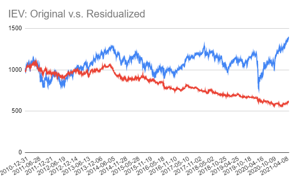
On this graph, the premium of being a European equity rather than a US, Japan or Emerging Markets equity clearly appears as negative over the whole observed period, and in nearly continuous erosion since 2014.
What to conclude?
First, if history repeats itself, any exposure of a portfolio to the European stock market to benefit from its idiosyncratic performances might be a drag on the portfolio returns, and should probably be avoided8.
But more importantly, if no risk premium exists to compensate investors for bearing the risk of specific exposure to the European stock market v.s. the other stock markets, why invest there?
Usage in portfolio factor exposures analysis
Another possible usage of residualization, particularly useful in portfolio factor exposures analysis, is to create uncorrelated factors in order to ease the interpretation of portfolio return contributions.
This is typically done in financial economics studies.
For example, Fama and French demonstrate1 that two bond-market factors TERM and DEF9 are present in stock returns in addition to the three stock-market factors RM-RF, SMB and HML.
To establish this result, they introduce the orthogonalized market factor RMO by residualizing the factor RM-RF on the factors SMB, HML, TERM and DEF. They then use this new factor to show that the two factors TERM and DEF capture strong common variation in stock returns, a property initially hidden due to the correlation of these factors with the factor RM-RF10.
Outside of academics, using residualization to create uncorrelated factors is also done in the asset management industry, for example in the Two Sigma Factor Lens product:
Though some factors are naturally orthogonal, we residualize our less liquid macro factors against more liquid ones to attempt to reduce correlations.
Two Sigma Factor Lens
Pitfalls
When only one factor is residualized, like in the examples above, understanding what residualization achieves is usually easy.
When several factors are residualized, though, the situation becomes more complex because residualization is not a simultaneous procedure.
Indeed, it needs to be decided which factor is residualized first, then second (on the remaining factors), then third (same), etc.1112, and different sequences of factors to residualize will generally lead to different interpretations of what residualization achieves.
In order to avoid this sequence dependence, one might be tempted to residualize all factors on one another.
Unfortunately, the residualized factors computed this way will in general not be uncorrelated, plus their interpretation will be difficult.
For example, the betas of the MSCI ACWI returns13 on both
- The MSCI World and MSCI Emerging Markets returns13
- The MSCI World and MSCI Emerging Markets residualized returns
over the period 2009/12/31 - 2021/05/28 are the following:
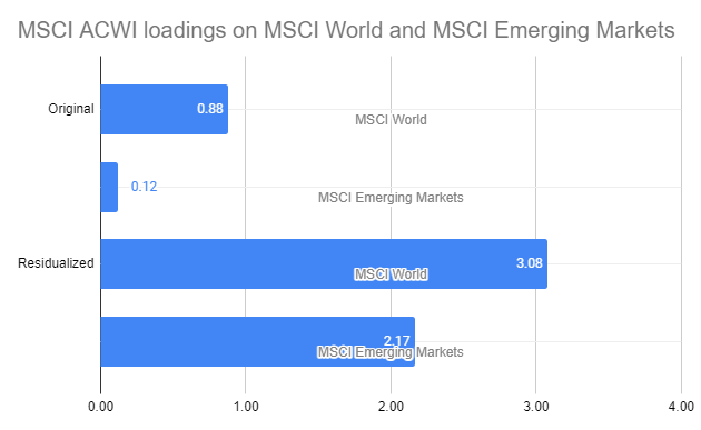
The interpretation of the betas on the MSCI World (88%) and on the MSCI Emerging Markets (12%) is rather easy: they correspond to the know weights of these indexes in the MSCI ACWI index14.
The interpretation of the betas on the residualized MSCI World (308%) and on the residualized MSCI Emerging Markets (217%) is a lot more difficult, even if the coefficient of determination of the associated linear regression analysis has exactly the same value of ~99.99%15!
So, what to do instead?
One possibility is to decorrelate all the factors at once, using mathematical techniques different from residualization.
This will be the subject of another post.
–
-
Fama, E.F., and K.R. French (1993),”Common Risk Factors in the Returns on Stocks and Bonds.” Journal of Financial Economics, Vol. 33, 3–56. ↩ ↩2
-
As well as generating other problems, for instance creating spurious risk contributions from the correlated factors, c.f. Meucci, Attilio and Santangelo, Alberto and Deguest, Romain, Risk Budgeting and Diversification Based on Optimized Uncorrelated Factors. ↩
-
Insofar as this is really a problem for the specific analysis to perform, c.f. for example Jan Vanhove, Collinearity isn’t a disease that needs curing. ↩
-
Catalina B. Garcia, Roman Salmeron, Claudia Garcia & Jose Garcia (2019): Residualization: justification, properties and application, Journal of Applied Statistics. ↩
-
For the geeks, orthogonality and uncorrelation are two different properties, c.f. Joseph Lee Rodgers; W. Alan Nicewander; Larry Toothaker, Linearly Independent, Orthogonal, and Uncorrelated Variables, The American Statistician, Vol. 38, No. 2. (May, 1984), pp. 133-134. The residuals obtained by ordinary least squares estimation will always be orthogonal to the observations of the explanatory variables, and they will also be uncorrelated if the regression model includes a constant or if the observations of the explanatory vcariables are centered. ↩
-
Non dividend-adjusted to match with FactorResearch data, obtained from Alpha Vantage. ↩
-
The same is not true for the graph of the residualized S&P500, probably because of differences in returns data. ↩
-
The residualized Europe equity factor is uncorrelated to the other equity factors per construction, so, no diversification effect would counterbalance the negative impact on returns. ↩
-
The TERM factor measures the exposure to unexpected changes in general interest rates and the DEF factor measures the exposure to the risk of corporate bond default. ↩
-
In Fama and French own words1, [RM-RF] is a hodgepodge of the common factors in returns. ↩
-
Mathematical quantities like the variance inflation factor (VIF), which quantifies the degree of multicollinearity in linear regression analysis (and which is computed using residualization!), can help in defining the sequence of explanatory variables to residualize. ↩
-
This sequential residualization procedure is sometimes labelled successive residualization4. ↩
-
Monthly gross returns in USD, obtained from the MSCI website. ↩ ↩2
-
At the date of publication of this post, from the MSCI website: The MSCI Emerging Markets(EM) Index was launched in 1988 including 10 countries with a weight of about 0.9% in the MSCI ACWI Index. Currently, it captures 26 countries across the globe and has a weight of 12% in the MSCI ACWI Index. ↩
-
Residualization has no impact on the coefficient of determination4. ↩