The Bogle Model for Bonds: Predicting the Returns of Constant Maturity Government Bond ETFs
In his original 1991 article Investing in the 1990s1, John Bogle described a simple model to help investors setting reasonable expectations for long-term U.S. government bond returns.
This model relies on what Bogle describes as the single most important factor in forecasting future total returns [of a government bond], which is the the initial yield to maturity.
In this post, I will describe Bogle’s methodology and analyze its forecasting performances when applied to constant maturity U.S. government bonds, which is a category of U.S. government bonds representative of most U.S. government bond ETFs as detailled in a previous post.
Bogle Sources of Return Model for Bonds (BSRM/B)
The Bogle Sources of Return Model for Bonds2 (BSRM/B) is a simple empirical model which states that there is but a single dominant source of decade-long returns on [government] bonds: the interest coupon2.
This model has initially been introduced by Bogle in the case of the 20-year U.S. Treasury bond1 and has then latter been shown to also be applicable in the case of the 10-year U.S. Treasury bond2.
Let’s dig into the details.
Forecasting performances for the 20-year U.S. Treasury bond
Bogle1 examines the relationship between the initial yield to maturity of a 20-year U.S. Treasury bond and its subsequent 10-year annualized total3 return, over the period 1930 - 1980.
He notices that1:
[…] in bonds, [the initial interest rate] is the single most important factor in forecasting future total returns. The other two factors are the reinvestment rate (the rate at which the interest coupons compound), and the terminal (or end-of-period) yield.
As a matter of fact, he later shows in his paper The 1990s at the Halfway Mark4 that these three factors taken together have a correlation of 0.99 with the actual returns on bonds in each of the decades4.
Now, because the reinvestment rate and the terminal yield are by definition unknown quantities, they cannot be used to forecast future bond returns, which leaves the initial interest rate as the critical variable, [which] has a correlation of 0.709 with the returns subsequently earned by bonds.1.
In other words, the initial yield to maturity of a 20-year U.S. Treasury bond is actually sufficient to explain substantially [the bond] […] return […] over the subsequent decade4.
Forecasting performances for the 10-year U.S. treasury bond
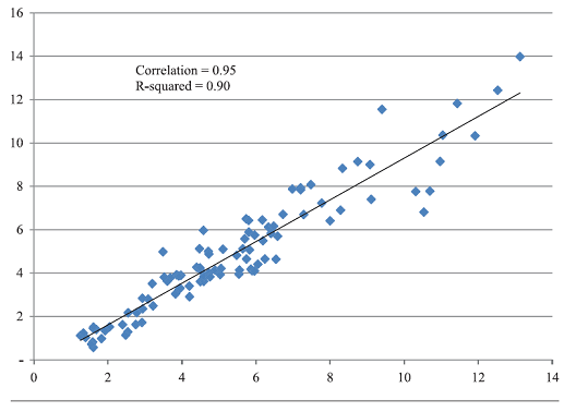
Bogle and Nolan2 examine the relationship between the initial yield to maturity of a 10-year U.S. Treasury bond and its subsequent 10-year annualized return over the period 1915–2014, and find that the initial interest rate explains ~90% of the variability of the subsequent 10-year annualized bond returns.
This finding is illustrated in Figure 1, directly reproduced from Bogle and Nolan2.
Forecasting performances, revisited
I propose to analyze the forecasting performances of the BSRM/B model when applied to constant maturity U.S. government bonds over the out-of-sample period 31th October 1993 - 31th May 2013.
Due to the close relationship between this category of U.S. government bonds and most U.S. government bond ETFs, this will help to understand if Bogle’s model could be of any practical use to today’s investors for setting long-term capital assumptions for U.S. government bonds.
Out-of-sample forecasting performances for the 20-year constant maturity U.S. Treasury bond
Using the monthly 20-Year Treasury Constant Maturity Rates series from the Federal Reserve website, Figure 2 shows that the initial yield to maturity at the end of any given month over the period 31th October 1993 - 31th May 2013 explains ~72.1% of the variability of the subsequent 10-year annualized bond returns.
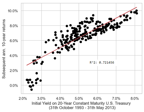
The associated monthly correlation coefficient is ~0.849, which is consistent with the yearly correlation coefficient of ~0.709 determined by Bogle1.
Out-of-sample forecasting performances for the 10-year constant maturity U.S. Treasury bond
Using the monthly 10-Year Treasury Constant Maturity Rates series from the Federal Reserve website, Figure 3 shows that the initial yield to maturity at the end of any given month over the period 31th October 1993 - 31th May 2013 explains ~85.2% of the variability of the subsequent 10-year annualized bond returns!
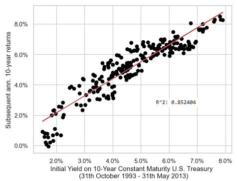
Such a value for the monthly $r^2$ coefficient is again consistent with the yearly $r^2$ coefficient of ~90% obtained by Bogle and Nolan2 and displayed in Figure 1.
Conclusion of the out-of-sample study
The empirical conclusions of this section are that:
- The BSRM/B model is definitely applicable to 20-year and 10-year constant maturity U.S. government bonds
- The out-of-sample forecasting performances of this model are similar to its in-sample forecasting performances5 for the two considered maturities
But what about the forecasting performances of the BSRM/B model for other maturities? For example, for the 3-year constant maturity U.S. government bond, represented in Figure 4, or for the 30-year constant maturity U.S. government bond, represented in Figure 5?
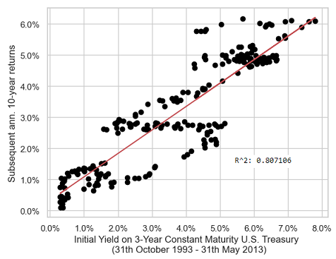
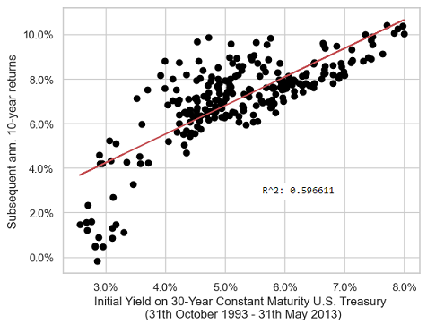
From Figure 2 to Figure 5, another empirical conclusion is that the BSRM/B model is best suited to a 10-year constant maturity U.S. government bond, because the more the deviation from a maturity of 10 years the more the degradation in forecasting performances6.
Forecasting performances, theoretical justification
Surprinsingly, all empirical conclusions of the previous section, and especially the last one, are backed up by theoretical results.
Indeed, Leibowitz et al.7 analyze the behaviour of constant duration bond funds and establish that multi-year […] returns […] converge in both mean and volatility around the starting yield7, with a convergence horizon of about $2D - 1$ years for a bond fund whose duration is $D$ years, regardless of interim changes in yields8 which only impact this convergence by widening the distribution of returns around the mean return7.
These results allow to understand the behaviour of the BSRM/B model when applied to the 10-year constant maturity U.S. government bond9:
- From its investable counterpart, the iShares 7-10 Year Treasury Bond ETF (IEF ETF), we can assume that its (constant-ish) duration is ~7.5 years at the date of publication of this post10
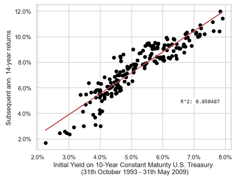
- From Leibowitz et al.7, we can then conclude that the initial yield to maturity of the 10-year constant maturity U.S. government bond should be predictive of its annualized returns over the subsequent ~2*7.5 - 1 = ~14 years, which is confirmed by Figure 6
- Nevertheless, again from Leibowitz et al.7, it can happen that the convergence horizon is much shorter in practice than in theory11, and it seems that this is exactly what happens for the 10-year constant maturity U.S. Treasury bond, with an effective convergence horizon of ~10 years (as confirmed by the very good forecasting performances depicted in Figure 3) v.s. a theoretical convergence horizon of ~14 years
These results also allow to understand the behaviour of the BSRM/B model when applied to the the 3-year, 20-year and 30-year constant maturity U.S. government bonds, as the initial yield to maturity of these bonds should then NOT be predictive of their annualized returns over the subsequent 10 years, but should rather be predictive of their annualized returns over the subsequent $2 D_3 - 1$, $2 D_{20} - 1$ and $2 D_{30} - 1$ years, with $D_3$, $D_{20}$ and $D_{30}$ their respective durations12.
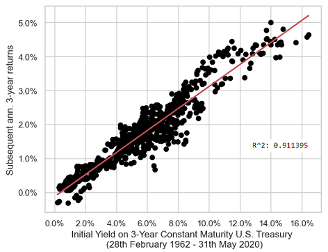
This theoretical behaviour is (somewhat) confirmed in practice, with for example Figure 7 illustrating that the initial yield to maturity of the 3-year constant maturity U.S. government bond is highly predictive of the annualized returns of this bond over the subsequent 3 years over the period 28th February 1962 - 31th May 2020.
Implementation in Portfolio Optimizer
A proprietary variation of Bogle’s BSRM/B model is implemented through the Portfolio Optimizer endpoint /markets/indicators/bsrmb/us to compute
- The initial yield of the U.S. 10-year constant maturity governement bond (i.e., the value of the BSRM/B model for this bond), over the 121 past months
- The forecasted 10-year annualized return for the U.S. 10-year constant maturity governement bond (investable asset - IEF ETF) and a 95% confidence interval around it, over the 121 future months
Examples of usage
Typical examples of usage for the BSRM/B model are similar to the ones described in a previous blog post about a predictor of long-term stock market returns called the AIAE.
For example:
- Setting long-term capital market assumptions for U.S. government bonds
As an illustration, Figure 8 displays the “path” of expected long-term returns for the 10-year constant maturity U.S. government bond over the period 28th February 1962 - 31th May 2023.
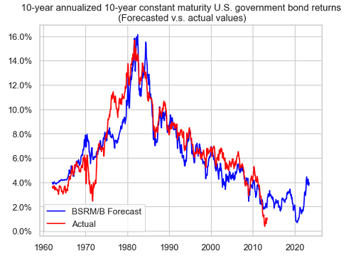
From Figure 8, and at the date of publication of this post13, a buy-and-hold investment in the 10-year constant maturity U.S. government bond is expected to yield an annualized return of ~4% over the next 10 years.
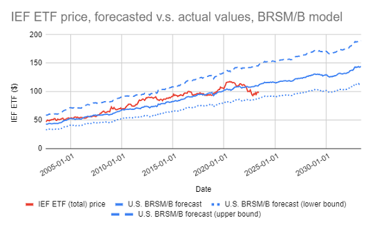
- Generating future price scenarios
Here, Figure 9 displays the price scenario corresponding to Figure 8 in the case of the IEF ETF, with a 95% confidence interval added.
A less typical example of usage would be to combine14 the forecasts produced by the BSRM/B model with estimations of the equity risk premium in order to predict future stock market returns.
A good starting place to find such estimations of the equity risk premium is the website of Aswath Damodaran, who maintains estimates of the historical implied equity risk premiums for the U.S. with plenty of details in his yearly-updated paper Equity Risk Premiums (ERP): Determinants, Estimation and Implications15.
Conclusion
Bogel’s bond model has proved very effective at predicting long-term U.S. governement bonds returns over more than thirty years after its initial publication, which confirms what Bogle1 wrote in his original paper:
when we know the current coupon, we know most of what we need to know to forecast [government] bond returns in the coming decade
I find this model is another interesting addition to one’s forecasting toolbox on top of the AIAE indicator!
For more forecasts, feel free to connect with me on LinkedIn or to follow me on Twitter.
–
-
See Bogle, J., Investing in the 1990s, The Journal of Portfolio Management, Vol. 17, No. 3 (1991a), pp. 5-14. ↩ ↩2 ↩3 ↩4 ↩5 ↩6 ↩7
-
See Bogle J., Nolan M., Occam’s Razor Redux: Establishing Reasonable Expectations for Financial Market Returns, Journal of Portfolio Management, Vol. 42, No. 101, Sep Fall 2015. ↩ ↩2 ↩3 ↩4 ↩5 ↩6
-
All bond returns considered in this blog post are total returns, so that I will omit “total”. ↩
-
See Bogle, J., The 1990s at the Halfway Mark, The Journal of Portfolio Management, Vol. 21, No. 4 (1995), pp. 21-31. ↩ ↩2 ↩3
-
More data is needed to support this claim here; for example, the in-sample monthly $r^2$ coefficient for the 10-year constant maturity U.S. Treasury bond is equal to ~83.9%, so that there is no apparent degradation of the BSRM/B model. ↩
-
This is especially visible in Figure 5, with an $r^2$ coefficient of only ~59.7%. ↩
-
See Martin L. Leibowitz, Anthony Bova & Stanley Kogelman (2014) Long-Term Bond Returns under Duration Targeting, Financial Analysts Journal, 70:1, 31-51. ↩ ↩2 ↩3 ↩4 ↩5
-
That is, whatever the pace of yield changes or the magnitude of yield changes. As a matter of fact, Leibowitz et al.7 show that what is important is the standard deviation of the yield change distribution. ↩
-
Viewing a constant maturity bond as a constant duration bond fund might seem as a leap of faith, but the analysis of constant duration bond funds done in Leibowitz et al.7 shows that they should not differ much in practice. ↩
-
The duration of the 10-year constant maturity U.S. Treasury bond/IEF ETF is not constant over time, so that this is a kind of first-order approximation. ↩
-
In Leibowitz et al.7, the effective convergence horizon of a 5-year constant duration bond fund is shown to 6 years instead of 9 years. ↩
-
Again, assumed to be constant in Leibowitz et al.7, which is not the case in practice. ↩
-
More precisely, assuming the investment starts on 31th May 2023. ↩
-
Of course, in a non-circular way. ↩
-
See Damodaran, Aswath, Equity Risk Premiums (ERP): Determinants, Estimation and Implications - The 2023 Edition. ↩