The Single Greatest Predictor of Future Stock Market Returns, Ten Years After
In his 2013 post The Single Greatest Predictor of Future Stock Market Returns, Jesse Livermore1 from the blog Philosophical Economics introduced an indicator to forecast long-term U.S. stock market returns and empirically demonstrated that it outperformed all the commonly used stock market valuation metrics like the Shiller CAPE2.
This indicator, called the Aggregate Investor Allocation to Equities (AIAE), has been further analyzed by Raymond Micaletti in his paper Towards a Better Fed Model3, with the conclusion that it indeed has superior equity-return forecasting ability compared to other well-known indicators (such as the CAPE ratio, Tobin’s Q, Market Cap-to-GDP, etc.)3.
In this post, I will describe in details the AIAE indicator, come back on nearly ten years of out-of-sample performances and show how to use the forecast procedure proposed by Micaletti3 in order to set long-term capital assumptions for the U.S. stock market.
The AIAE indicator
Definition
Livermore4 defines the AIAE indicator as the total amount of stocks that investors are holding in aggregate divided by the total amount of stocks plus bonds plus cash that these same investors are holding in aggregate, that is
\[AIAE = \frac{TMV_s}{TMV_s + TMV_b + C}\], where:
- $TMV_s$ is the total market value of stocks
- $TMV_b$ is the total market value of bonds
- $C$ is the total market value of cash
By definition, this indicator represents the average investor allocation to stocks5, hence its name.
Computation of the U.S. AIAE indicator
Through some approximations, Livermore4 shows that it is possible to compute the AIAE indicator for the U.S. thanks to economic data published in the quarterly Federal Reserve release Financial Accounts of the United States - Z.1.
In details:
- The total market value of stocks $TMV_s$ is approximated by the sum of
- The market value of non-financial corporate businesses - Fred data series Nonfinancial Corporate Business; Corporate Equities; Liability, Level (NCBEILQ027S)
- The market value of financial corporate businesses - Fred data series Domestic Financial Sectors; Corporate Equities; Liability, Level (FBCELLQ027S)
- The total market value of bonds plus cash $TMV_b + C$ is approximated by the sum of the total liabilities of real economic borrowers, that is
- The liabilities of the federal government - Fred data series Federal Government; Debt Securities and Loans; Liability, Level (FGSDODNS)
- The liabilities of households and nonprofit organizations - Fred data series Households and Nonprofit Organizations; Debt Securities and Loans; Liability, Level (CMDEBT)
- The liabilities of non-financial corporate businesses - Fred data series Nonfinancial Corporate Business; Debt Securities and Loans; Liability, Level (BCNSDODNS)
- The liabilities of the rest of the world - Fred data series Rest of the World; Debt Securities and Loans; Liability, Level (DODFFSWCMI)
- The liabilities of the state and local governments - Fred data series State and Local Governments; Debt Securities and Loans; Liability, Level (SLGSDODNS)
The U.S. AIAE indicator computed using the above Fred data series is available -> here.
Forecasting performances of the U.S. AIAE indicator
Figure 1, adapted from Livermore4, compares the value of the U.S. AIAE indicator at the end of any given quarter over the period 31th December 1951 - 30th September 20036 with the subsequent 10-year annualized S&P 500 total7 returns.
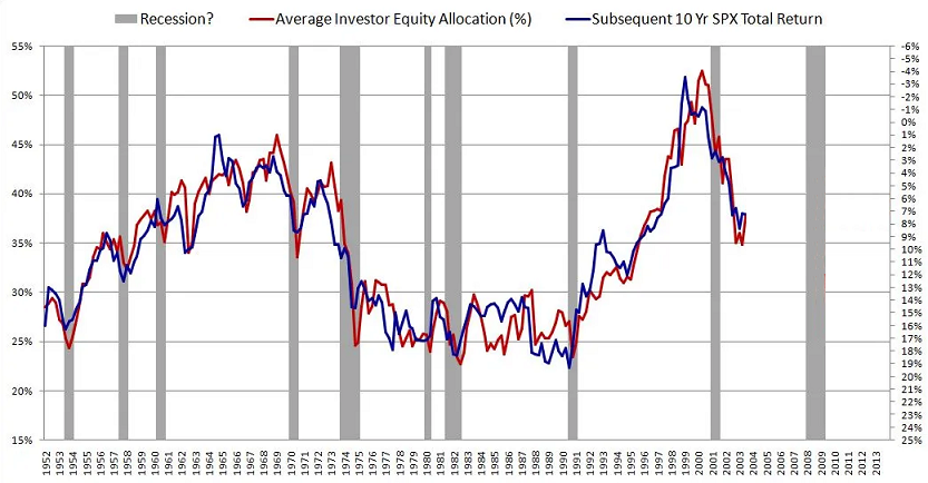
It appears that this indicator is doing an impressive job at predicting future U.S. stock market returns!
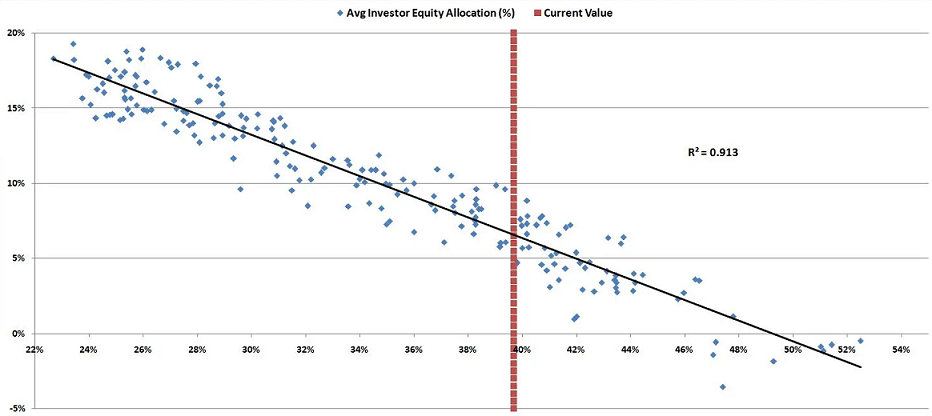
This can be confirmed more formally through an ordinary least square regression.
Figure 2, directly reproduced from Livermore4, shows that the value of the U.S. AIAE indicator at the end of any given quarter over the period 31th December 1951 - 30th September 20036 explains ~91.3% of the variability of the subsequent 10-year annualized S&P 500 returns.
These compelling forecasting performances need nevertheless to be taken with a grain of salt, because they are not exactly achievable in real life due to two problems:
- First, the implicit hindsight bias associated to Figure 1 and Figure 2
This problem is discussed more in details for example in Asness et al.8 in the case of the CAPE ratio, but it suffices to say that many equity valuation indicators usually present both encouraging in-sample long-horizon [performance]8 and directionally right but weak and disappointing out-of-sample performance8.
One solution to this problem is to evaluate the forecasting performances of equity valuation indicators in a kind of walk-forward fashion.
For the U.S. AIAE indicator, this is done in Micaletti3, who conclude that
the Aggregate Investor Allocation to Equities (AIAE) has superior equity-return forecasting ability compared to other well-known indicators (such as the CAPE ratio, Tobin’s Q, Market Cap-to-GDP, etc.)
More on this in the next section.
- Second, Fred data revisions
After the initial release of economic data (unemployment, GDP, etc.), it is usual to see these data being revised a couple of weeks, months, or quarters later.
So, because the AIAE indicator is based on economic data, its value on a given past date as computed today v.s. as computed just after the initial release of the associated economic data might be different.
Hopefully, there are some hints in Micaletti3 that the impact of this problem might be neglictible in practice.
Rationale of the U.S. AIAE indicator
Livermore4 argues that, under reasonable assumptions, long-term stock market returns must be driven by dynamics in equities supply v.s. bonds plus cash supply, dynamics that are precisely captured by the AIAE indicator.
I will not repeat his whole reasoning here9, but it shares some similarities with the reasoning of Sharpe in his paper The Arithmetic of Active Management10 in that it uses arithmetic arguments to model the behaviour of an imaginary “aggregate investor”.
Forecasting performances of the U.S. AIAE indicator, revisited
In this section, I will study the forecasting performances of the U.S. AIAE indicator since its publication.
Because Livermore published the associated blog post on 20th December 20134, he had access to
- Fred economic data for the period 31th December 1951 - 30th September 2013
- S&P 500 return data up to 20th December 2013
, which allowed him to analyze the 10-year forecasting performances of the U.S. AIAE indicator over the period 31th December 1951 - 30th September 2003.
On my side, at the date of publication of this post, I have access to
- Fred economic data for the period 31th December 1951 - 31th December 2022
- S&P 500 return data up to 22th May 2023
, which allows me to analyze the 10-year forecasting performances of the U.S. AIAE over the additional out-of-sample period 31th December 2003 - 31th March 2013.
I will use two methodologies:
- The methodology of Livermore4, which consists in computing all pairs (U.S. AIAE indicator, realized subsequent 10-year annualized U.S. stock market returns) over the period 31th December 1951 - 31th March 2013
- The methodology of Micaletti3, which consists in
- Computing all pairs (U.S. AIAE indicator, realized subsequent 10-year annualized U.S. stock market returns) over the expanding period 31th December 1951 - $t$, $t$ = 31th December 1961,…, 31th March 2003
- Fitting a linear least square regression line on these pairs
- Extracting the associated linear regression coefficients $\alpha_t$ and $\beta_t$
- Forecasting the 10-year annualized U.S. stock market return from $t + 10$ years to $t + 20$ years by the formula $ \alpha_t + \beta_t AIAE_t $, where $AIAE_t$ is the value of the U.S. AIAE indicator on date $t$
Data
The data sources for this study are the following:
- The Alfred website, for Fred economic data (I used initial releases only11)
- The Kenneth French’s website, for U.S. stock market returns
To be noted that it is possible to access Alfred economic data through a well-documented Web API.
Livermore’s methodology (in-sample forecasting performances)
31th December 1951 - 30th September 2003
Figure 3 is my reproduction of Figure 2 from Livermore4.
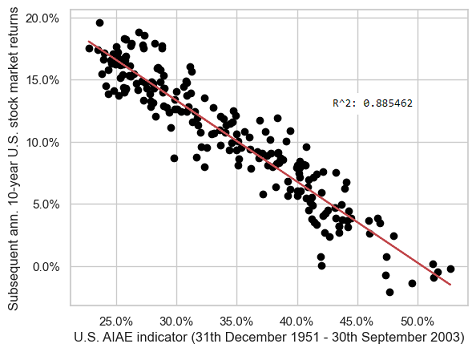
Although there is a slight difference in the $r^2$ coefficients (~91.3% in Figure 2 v.s. ~88.5% in Figure 3), probably related to differences in both Fred data12 and U.S. stock market return data13, these two figures look very much alike.
This validates my reproduction of Livermore’s methodology.
31th December 2003 - 31th March 2013
Figure 4 is the same as Figure 3, with the data points corresponding to the out-of-sample period 31th December 2003 - 31th March 2013 added.
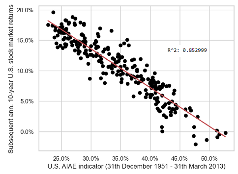
Unfortunately, the $r^2$ coefficient has decreased (from ~88.5% in Figure 3 to ~85.2% in Figure 4), which implies that forecasting performances have degraded over the most recent period.
This is confirmed by Figure 5, which displays only the data points corresponding to the out-of-sample period.
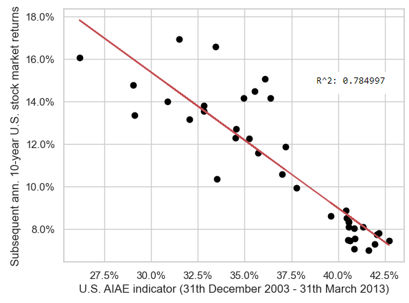
On this figure, it is clearly visible that the relationship between the U.S. AIAE indicator and the subsequent 10-year annualized U.S. stock market returns is linear-ish, but with a high variability.
Micaletti’s methodology (walk-forward forecasting performances)
31th December 1951 - 30th September 2003
Figure 6 empirically demonstrates that the forecasts of the 10-year annualized U.S. stock market returns obtained using Micaletti’s methodology3 match extremely well with their actual counterparts over the period 31th December 1951 - 30th September 2003.
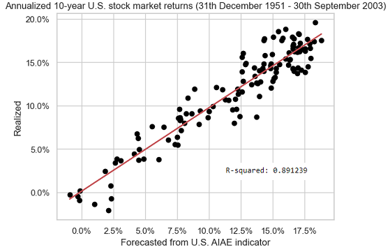
As a side note, the $r^2$ coefficient obtained with the “real-time” methodology of Micaletti (~89.1% in Figure 6) is a little bit higher than the $r^2$ coefficient obtained using the “hindsight-biased” methodology of Livermore (~88.5% in Figure 3).
This might be linked to the usage of an expanding window in Micaletti’s methodology, which allows to account for dynamics in the evolution of the linear regression coefficients, or this might more probably just be noise.
31th December 2003 - 31th March 2013
Figure 7 is the same as Figure 6, with the data points corresponding to the out-of-sample period 31th December 2003 - 31th March 2013 added.
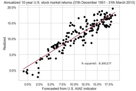
The situation here is the same as with Livermore’s methodology, that is, the $r^2$ coefficient has decreased over the most recent period (from ~89.1% in Figure 6 to ~84.1% in Figure 7).
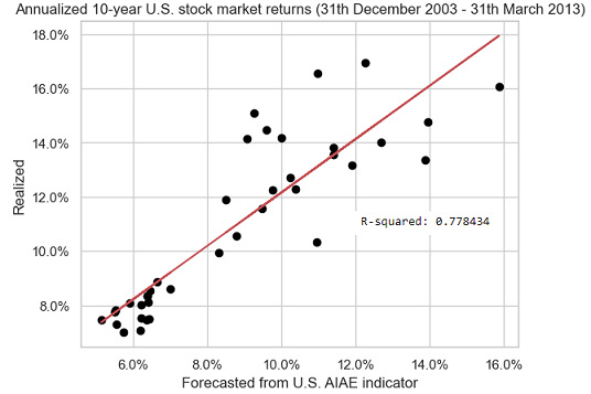
The associated degradation in forecasting performances is confirmed in Figure 8, which displays only the data points corresponding to the out-of-sample period.
Conclusion of the out-of-sample study
The bottom line of what precedes is that the forecasting performances of the U.S. AIAE indicator have indubitably decreased since its publication by Livermore4, which is materialized by a lower $r^2$ coefficient.
While the COVID crisis and recovery certainly played a role, it is actually not the first time in history that such a decrease in forecasting performances occurs.
Figure 9 displays the rolling $r^2$ coefficient, over a prior period of 10 years, of the 10-year annualized U.S. stock market returns forecasts v.s. actual values.
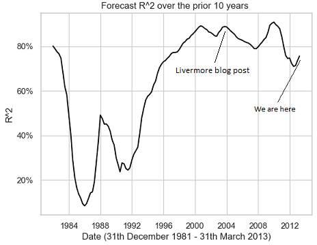
On this figure, there are many 10-year periods with an $r^2$ coefficient much lower than ~77.8%, with even 10-year periods whose $r^2$ coefficient is much lower than 20%!!
So, as glimmers of hope, 1) there have been much worse underperforming periods in history than the current one (relative hope) and 2) the current $r^2$ coefficient is still very high for an equity valuation indicator4 (absolute hope).
Implementation in Portfolio Optimizer
A proprietary variation of Micaletti’s methodology3 is implemented through the Portfolio Optimizer endpoint /markets/indicators/aiae/us to compute:
- The U.S. AIAE, over the 41 past quarters
- The forecasted 10-year annualized U.S. stock market return (investable asset - SPY ETF) and a 95% confidence interval around it, over the 41 future quarters
Examples of usage
Setting (better) long-term capital market assumptions for the U.S. stock market
Every year, major financial institutions publish their long-term capital market assumptions based on their internal valuation models (BlackRock, J.P.Morgan…).
The U.S. AIAE indicator enables individual investors to have access to such a valuation model in the case of the U.S. stock market.
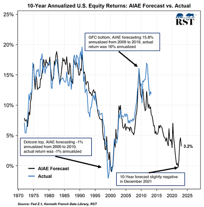
Even better, the U.S. AIAE indicator also enables individual investors to have access to the “path” of expected long-term U.S. stock market returns, as for example regularly published by Micaletti on his twitter account through images like Figure 10.
For comparison (shameless plug):
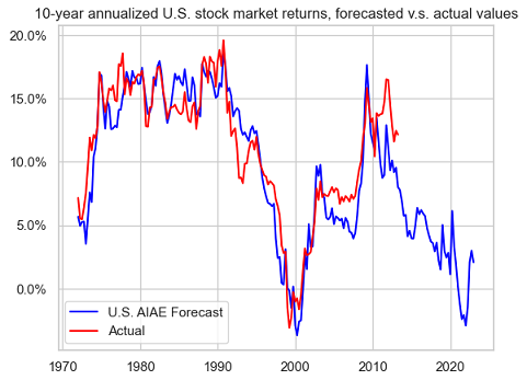
- The path equivalent to Figure 10, but generated by Portfolio Optimizer, is depicted in Figure 11.
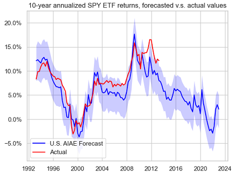
- The same path as in Figure 11, with 95% confidence interval and using the SPY ETF returns, is depicted in Figure 12.
Thanks to these forecasts, it becomes possible to contextualize the long-term capital market assumptions of financial institutions.
For example:
- BlackRock forecast14 a 10-year annualized U.S. stock market return from 31th December 2022 to 31th December 2032 of ~7.9%.
This forecast can be compared to the U.S. AIAE forecast of ~2.1% in Figure 12 and of not a much higher value in Figure 11.
- J.P.Morgan comment15 on December 2022 that
Lower valuations and higher yields mean that markets today offer the best potential long-term returns since 2010
This comment can be put into perspective by looking at the U.S. AIAE forecasts around 2010 in Figure 12 and Figure 11.
Generating future price scenarios for the SPY ETF
The U.S. AIAE forecasts of long-term U.S. stock market returns can be converted into future price scenarios for misc. traded instruments.
In the case of the SPY ETF, the price scenarios corresponding to Figure 12 are represented in Figure 13.
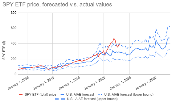
Such price scenarios are sometimes more easy to grasp, or to describe to customers, than forecasts of pure returns.
Looking at Figure 13, it is for example clear that the price of the SPY ETF is currently not where it “should” be, and that, assuming the U.S. AIAE indicator continues to be reliable, we might be in for at best ~2 years of flat returns and at worst for a moderate to severe U.S. market correction anytime soon…
Tactical asset allocation
The forecasts generated by the U.S. AIAE indicator can also be used within a tactical asset allocation framework, as detailed for example in Micaletti3, who note that:
[…] over the last 43 years and across various subperiods, the AIAE-based TAA strategy delivered the most consistently high-level performance relative to its competitors.
Alternatively, they could also be integrated in any other tactical asset allocation framework that already uses an equity valuation indicator, like the framework described in Asness et al.8.
I will not go into more details here, though.
Conclusion
Nearly one decade of out-of-sample forecasting performances validates that the AIAE indicator introduced by Livermore4 has been very impressive in the U.S.
Now, whether the current period of (relative) underperformance will continue or stop in the future is of course open to debate, but in any cases, I hope that this blog post shed some light on this little-known equity valuation indicator.
For more uncommon quantitative nuggets, feel free to connect with me on LinkedIn or to follow me on Twitter.
–
-
This is a pseudonym. ↩
-
See Campbell, John Y., Robert J. Shiller (1988a). Stock prices, earnings, and expected dividends. Journal of Finance 43, 661-676. ↩
-
See Micaletti, Raymond, Towards a Better Fed Model. ↩ ↩2 ↩3 ↩4 ↩5 ↩6 ↩7 ↩8 ↩9
-
See The Single Greatest Predictor of Future Stock Market Returns. ↩ ↩2 ↩3 ↩4 ↩5 ↩6 ↩7 ↩8 ↩9 ↩10 ↩11
-
Livermore4 makes the working assumption that an investor can only invest in stocks, bonds or cash as far as financial assets are concerned; whether the development of alternative financial asset classes like cryptocurrencies will at some point impact this assumption remains to be seen. ↩
-
Although there is no reference in Livermore4 to the exact period used for his graphs, my best guess is 31th December 1951 - 30th September 2003. ↩ ↩2
-
All stock market returns considered in this blog post are total returns, so that I will omit “total”. ↩
-
See Cliff Asness, Antti Ilmanen and Thomas Maloney, Market Timing: Sin a Little Resolving the Valuation Timing Puzzle, Journal Of Investment Management, Volume 15, Number 3, 2017. ↩ ↩2 ↩3 ↩4
-
See William F. Sharpe, The Arithmetic of Active Management, Financial Analysts Journal, Vol. 47, No. 1 (Jan. - Feb., 1991), pp. 7-9. ↩
-
The Alfred website is a point in time version of the Fred website, which allows to access initial releases or more generally specific point in time versions of economic data. ↩
-
There is no reference in Livermore4 to whether the Fred data are initial releases, but my best guess is that they are not. ↩
-
I used the stock market returns provided on the Kenneth French’s website, while Livermore4 used the S&P 500 returns. ↩
-
See BlackRock website. ↩