Simulation from a Multivariate Normal Distribution with Exact Sample Mean Vector and Sample Covariance Matrix

In the research report Random rotations and multivariate normal simulation¹, Robert Wedderburn introduced an algorithm to simulate i.i.d. samples from a multivariate normal (Gaussian) distribution when the desired sample mean vector and sample covariance matrix are known in advance².

Wedderburn unfortunately never had the opportunity to publish his report³ and his work was forgotten until Li⁴ rediscovered it nearly 20 years later.

In this short blog post, I will first describe the standard algorithm used to simulate i.i.d. samples from a multivariate normal distribution and I will then detail Wedderburn’s original algorithm as well as some of the modifications proposed by Li.

Mathematical preliminaries

Affine transformation of a multivariate normal distribution

A textbook result related to the multivariate normal distribution is that any linear combination of normally distributed random variables is also normally distributed.

More formally:

Property 1: Let $X$ be a n-dimensional random variable following a multivariate normal distribution $\mathcal{N} \left( \mu, \Sigma \right)$ of mean vector $\mu \in \mathbb{R}^{n}$ and of covariance matrix $\Sigma \in \mathcal{M}(\mathbb{R}^{n \times n})$. Then, any affine transformation $Z = AX + b$ with $A \in \mathcal{M}(\mathbb{R}^{n \times m})$ and $b \in \mathbb{R}^{m}$, $m \ge 1$, follows a m-dimensional multivariate normal distribution $\mathcal{N} \left( A \mu + b, A \Sigma A {}^t \right)$.

Orthogonal matrices

An orthogonal matrix of order $n$ is a matrix $Q \in \mathcal{M}(\mathbb{R}^{n \times n})$ such that $Q {}^t Q = Q Q {}^t = \mathbb{I_n}$, with $\mathbb{I_n}$ the identity matrix of order $n$.

By extension, a rectangular orthogonal matrix is a matrix $Q \in \mathcal{M}(\mathbb{R}^{m \times n}), m \geq n$ such that $Q {}^t Q = \mathbb{I_n}$.

Random orthogonal matrices

A random orthogonal matrix of order $n$ is a random matrix $Q \in \mathcal{M}(\mathbb{R}^{n \times n})$ distributed according to the Haar measure over the group of orthogonal matrices, c.f. Anderson et al.⁵.

By extension, a random rectangular orthogonal matrix is a matrix $Q \in \mathcal{M}(\mathbb{R}^{m \times n}) , m \geq n$, whose columns are, for example, the first $n$ columns of a random orthogonal matrix of order $m$, c.f. Li⁴.

Helmert orthogonal matrices

An Helmert matrix of order $n$ is a square orthogonal matrix $H \in \mathcal{M}(\mathbb{R}^{n \times n})$ having a prescribed first row and a triangle of zeroes above the diagonal⁶.

For example, the matrix $H_n$ defined by

\[H_n = \begin{pmatrix} \frac{1}{\sqrt n} &\frac{1}{\sqrt n} & \frac{1}{\sqrt n} & \dots & \frac{1}{\sqrt n} \\ \frac{1}{\sqrt 2} & -\frac{1}{\sqrt 2} & 0 & \dots & 0 \\ \frac{1}{\sqrt 6} & \frac{1}{\sqrt 6} & -\frac{2}{\sqrt 6} & \dots & 0 \\ \vdots & \vdots & \vdots & \vdots & \vdots\\ \frac{1}{\sqrt { n(n-1) }} & \frac{1}{\sqrt { n(n-1) }} & \frac{1}{\sqrt { n(n-1) }} &\dots & -\frac{n-1}{\sqrt { n(n-1) }} \end{pmatrix}\]

is a Helmert matrix.

A generalized Helmert matrix of order $n$ is a square orthogonal matrix $G \in \mathcal{M}(\mathbb{R}^{n \times n})$ that can be transformed by permutations of its rows and columns and by transposition and by change of sign of rows, to a form of a [standard] Helmert matrix⁶.

For example, the matrix $G_n$ defined by

\[G_n = \begin{pmatrix} \frac{1}{\sqrt n} &\frac{1}{\sqrt n} & \frac{1}{\sqrt n} & \dots & \frac{1}{\sqrt n} \\ -\frac{1}{\sqrt 2} & \frac{1}{\sqrt 2} & 0 & \dots & 0 \\ -\frac{1}{\sqrt 6} & -\frac{1}{\sqrt 6} & \frac{2}{\sqrt 6} & \dots & 0 \\ \vdots & \vdots & \vdots & \vdots & \vdots\\ -\frac{n-1}{\sqrt { n(n-1) }} & -\frac{1}{\sqrt { n(n-1) }} & -\frac{1}{\sqrt { n(n-1) }} &\dots & \frac{n-1}{\sqrt { n(n-1) }} \end{pmatrix}\]

is a generalized Helmert matrix, obtained from the matrix $H_n$ by change of sign of rows $i=2..n$.

Simulation from a multivariate normal distribution

Let be:

• $n$ a number of random variables⁷
• $\mu \in \mathbb{R}^{n}$ a vector
• $\Sigma \in \mathcal{M} \left( \mathbb{R}^{n \times n} \right)$ a positive semi-definite matrix

One of the most well known algorithm to generate $m \geq 1$ i.i.d. samples $X_1, …, X_m$ from the $n$-dimensional multivariate normal distribution $\mathcal{N}(\mu, \Sigma)$ relies on the Cholesky decomposition of the covariance matrix $\Sigma$.

Algorithm

In details, this algorithm is as follows:

• Compute the⁸ Cholesky decomposition of $\Sigma$
  • This gives $\Sigma = L L {}^t$, with $L \in \mathcal{M} \left( \mathbb{R}^{n \times n} \right)$ a lower triangular matrix
• Generate $m$ i.i.d. samples $Z_1,…, Z_m$ from the standard $n$-dimensional multivariate normal distribution $\mathcal{N}(0, \mathbb{I_n})$
  • This is done by generating $m \times n$ i.i.d. samples $z_{11}, z_{21}, …, z_{n1}, z_{1m}, z_{2m}, …, z_{nm}$ from the standard univariate normal distribution $\mathcal{N}(0, 1)$ and re-organizing these samples in $m$ vectors of $n$ variables $Z_1 = \left( z_{11}, z_{21}, …, z_{n1} \right) {} ^t, …, Z_m = \left( z_{1m}, z_{2m}, …, z_{nm} \right) {} ^t$
• Transform the samples $Z_1,…, Z_m$ into the samples $X_1,…,X_m$ using the affine transformation $X_i = L Z_i + \mu, i = 1..m$
  • From Property 1, $X_1,…,X_m$ are then $m$ i.i.d. samples from the multivariate normal distribution $\mathcal{N}(\mu, \Sigma)$

Theoretical moments v.s. sample moments

When the previous algorithm is used to generate $m$ i.i.d. samples $X_1, …, X_m$ from the $n$-dimensional multivariate normal distribution $\mathcal{N}(\mu, \Sigma)$, the sample mean vector

\[\bar{X} = \frac{1}{m} \sum_{i = 1}^m X_i\]

and the (unbiased) sample covariance matrix

\[Cov(X) = \frac{1}{m-1} \sum_{i = 1}^m \left(X_i - \bar{X} \right) \left(X_i - \bar{X} \right) {}^t\]

will be different from their theoretical counterparts, as illustrated in Figure 1 with $\mu = \left( 0, 0 \right){}^t$, $\Sigma = \begin{bmatrix} 3 & 1 \newline 1 & 2 \end{bmatrix}$ and $m = 250$.

Figure 1. Simulation from a multivariate normal distribution, first two sample moments v.s. first two theoretical moments.

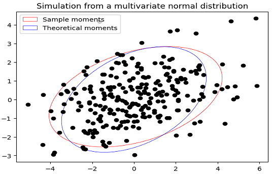
While convergence of the first two sample moments toward the first two theoretical moments is guaranteed when $m \to +\infty$, their mismatch for finite $m$ is usually⁹ an issue in practical applications.

Indeed, a large number of samples is then usually required in order to reach a reasonable level of accuracy for whatever statistical estimator is being computed, and generating such a large number of samples is costly in computation time.

Simulation from a multivariate normal distribution with exact sample mean vector and sample covariance matrix

Let be:

• $n$ a number of random variables⁷
• $\bar{\mu} \in \mathbb{R}^{n}$ a vector
• $\bar{\Sigma} \in \mathcal{M} \left( \mathbb{R}^{n \times n} \right)$ a positive definite matrix

Wedderburn’s algorithm¹ is a conditional Monte Carlo algorithm to generate multivariate normal samples conditional on a given mean and dispersion matrix¹.

In other words, given a desired sample mean vector $\bar{\mu}$ and a desired (unbiased) sample covariance matrix $\bar{\Sigma}$, Wedderburn’s algorithm allows to generate $m \geq n + 1$ i.i.d. samples $X_1, …, X_m$ from a $n$-dimensional multivariate normal distribution satisfying the two relationships

\[\bar{X} = \frac{1}{m} \sum_{i = 1}^m X_i = \bar{\mu}\]

and

\[Cov(X) = \frac{1}{m-1} \sum_{i = 1}^m \left(X_i - \bar{X} \right) \left(X_i - \bar{X} \right) {}^t = \bar{\Sigma}\]

By enforcing an exact match for finite $m$ between the first two sample moments and the first two theoretical moments of a multivariate normal distribution, Wedderburn’s algorithm allows to reduce the number of samples required in order to reach a reasonable level of accuracy for whatever statistical estimator is being computed, hence the total computation time¹⁰.

From this perspective, Wedderburn’s algorithm can be considered as a Monte Carlo variance reduction technique.

Wedderburn’s algorithm

In details, Wedderburn’s algorithm is as follows¹⁴:

• Generate a random rectangular orthonormal matrix $P \in \mathcal{M} \left( \mathbb{R}^{(m-1) \times n} \right)$, with $m \geq n + 1$
• Compute the⁸ Cholesky decomposition of the matrix $\bar{\Sigma}$
  • This gives $\bar{\Sigma} = L L {}^t$, with $L \in \mathcal{M} \left( \mathbb{R}^{n \times n} \right)$ a lower triangular matrix
• Define $X = \sqrt{m-1} T {}^t P L {}^t + \mathbb{1}_{m} \bar{\mu} {}^t$, with $T \in \mathcal{M} \left( \mathbb{R}^{(m-1) \times m} \right)$ made of the last $m-1$ rows of the $m \times m$ generalized Helmert matrix $G_n$ and $\mathbb{1}_{m} \in \mathbb{R}^{m}$ a vector made of ones
  • The rows $X_1, …, X_m$ of $X \in \mathcal{M} \left( \mathbb{R}^{m \times n} \right)$ are then $m$ i.i.d. samples from a multivariate normal distribution whose sample mean vector is equal to $\bar{\mu}$ and whose (unbiased) sample covariance matrix is equal to $\bar{\Sigma}$

Li’s modifications of Wedderburn’s algorithm

Li⁴ proposes several modifications to the original Wedderburn’s algorithm and show in particular how to manage a positive semi-definite covariance matrix $\bar{\Sigma}$.

In details, Wedderburn-Li’s algorithm is as follows⁴:

• Let $1 \leq r \leq n$ be the rank of the desired (unbiased) sample covariance matrix $\bar{\Sigma}$
• Generate a random rectangular orthonormal matrix $P \in \mathcal{M} \left( \mathbb{R}^{(m-1) \times r} \right)$, with $m \geq r + 1$
• Compute the⁸ reduced Cholesky decomposition of the matrix matrix $\bar{\Sigma}$
  • This gives $\bar{\Sigma} = L L {}^t$, with $L \in \mathcal{M} \left( \mathbb{R}^{n \times r} \right)$ a “lower triangular” matrix
• Define $X = \sqrt{m-1} T {}^t P L {}^t + \mathbb{1}_{m} \bar{\mu}$, with $T \in \mathcal{M} \left( \mathbb{R}^{(m-1) \times m} \right)$ made of the last $m-1$ rows of the $m \times m$ generalized Helmert matrix $G_n$ and $\mathbb{1}_{m} \in \mathbb{R}^{m}$ a vector made of ones
  • The rows $X_1, …, X_m$ of $X \in \mathcal{M} \left( \mathbb{R}^{m \times n} \right)$ are then $m$ i.i.d. samples from a multivariate normal distribution whose sample mean vector is equal to $\bar{\mu}$ and whose (unbiased) sample covariance matrix is equal to $\bar{\Sigma}$

Misc. remarks

A couple of remarks:

• Contrary to the algorithm described in the previous section, it appears at first sight that no sample from the univariate standard normal distribution $\mathcal{N}(0, 1)$ needs to be generated when using Wedderburn’s algorithm.

  This is actually not the case, because generating a random orthogonal matrix implicitely relies on the generation of such samples!

• Wedderburn¹ uses the eigenvalue decomposition of the covariance matrix $\bar{\Sigma}$ instead of its Cholesky decomposition, but Li⁴ demonstrates that it is actually possible to use any decomposition of $\bar{\Sigma}$ such that $\bar{\Sigma} = A A {}^t$ with $A \in \mathcal{M} \left( \mathbb{R}^{n \times n} \right)$ and advocates for the usage of the Cholesky decomposition.

• As highlighted in Wedderburn¹, the theoretical mean vector and covariance matrix of the multivariate normal distribution are irrelevant.

Implementation in Portfolio Optimizer

Portfolio Optimizer implements both the standard algorithm and Wedderburn-Li’s algorithm to simulate from a multivariate normal distribution through the endpoint /assets/returns/simulation/monte-carlo/gaussian/multivariate.

To be noted, though, that for internal consistency reasons, the input covariance matrix when using Wedderburn-Li’s algorithm is assumed to be the desired biaised sample covariance matrix and not the desired unbiased sample covariance matrix.

Conclusion

To conclude this post, a word about applications of Wedderburn’s algorithm.

These are of course numerous in finance, c.f. for example applications of similar Monte Carlo variance reduction techniques in asset pricing in Wang¹¹ or in risk management in Meucci¹².

But Wedderburn’s algorithm is applicable in any context requiring the simulation from a multivariate normal distribution, which makes it a very interesting generic algorithm to have in one’s toolbox!

For more analysis of forgotten research reports and algorithms, feel free to connect with me on LinkedIn or to follow me on Twitter.

–

1. See Wedderburn, R.W.M. (1975), Random rotations and multivariate normal simulation. Research Report, Rothamsted Experimental Station. ↩ ↩² ↩³ ↩⁴ ↩⁵ ↩⁶

2. That is, the samples are simulated so that they have the desired sample mean and sample covariance matrix. ↩

3. Because he died suddenly in 1975… ↩

4. See K.-H. Li, Generation of random matrices with orthonormal columns and multivariate normal variates with given sample mean and covariance, J. Statist. Comput. Simulation 43 (1992) 11–18. ↩ ↩² ↩³ ↩⁴ ↩⁵ ↩⁶

5. See T. W. Anderson, I. Olkin, L. G. Underhill, Generation of Random Orthogonal Matrices, SIAM Journal on Scientific and Statistical ComputingVol. 8, Iss. 4 (1987). ↩

6. See H. O. Lancaster, The Helmert Matrices, The American Mathematical Monthly, 72(1965), no. 1, 4-12. ↩ ↩²

7. On this blog such variables are typically assets, but they can also be genes or species in a biology context, etc. ↩ ↩²

8. In case a matrix is positive definite, its Cholesky decomposition exists and is unique; in case a matrix is only positive semi-definite, its Cholesky decomposition exists but is not unique in general. ↩ ↩² ↩³

9. Not always, as variability in the sample mean and in the sample covariance matrix might be desired. ↩

10. Under the assumption that the total time taken to generate this reduced number of samples + to compute the associated estimator is (much) lower than the total time taken to generate the initial larger number of samples + to compute the associated estimator. ↩

11. See Jr-Yan Wang, Variance Reduction for Multivariate Monte Carlo Simulation, The Journal of Derivatives Fall 2008, 16 (1) 7-28. ↩

12. See Meucci, Attilio, Simulations with Exact Means and Covariances (June 7, 2009). ↩