Supervised Portfolios: A Supervised Machine Learning Approach to Portfolio Optimization

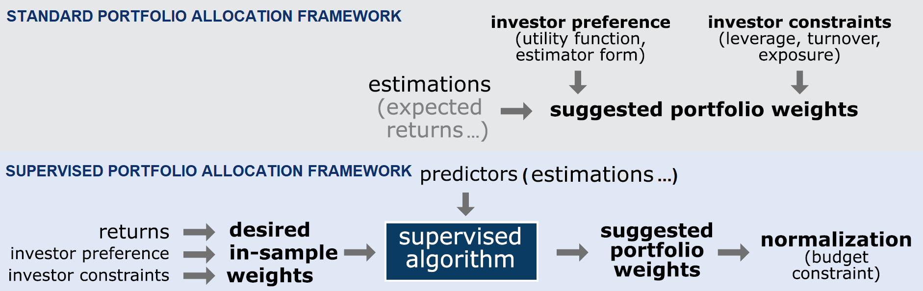
Standard portfolio allocation algorithms like Markowitz mean-variance optimization or Choueffati diversification ratio optimization usually take in input asset information (expected returns, estimated covariance matrix…) as well investor constraints and preferences (maximum asset weights, risk aversion…) to produce in output portfolio weights satisfying a selected mathematical objective like the maximization of the portfolio Sharpe ratio or Diversification ratio.

Chevalier et al.¹ introduces a non-standard portfolio allocation framework - represented in Figure 1 - under which the same input is first used to “learn” in-sample optimized portfolio weights in a supervised training phase and then used to produce out-of-sample optimized portfolio weights in an inference phase.

Figure 1. Standard v.s. supervised portfolio allocation framework. Source: Adapted from Chevalier et al.

In this blog post, I will provide some details about that framework when used with the $k$-nearest neighbors supervised machine learning algorithm, which is an idea originally proposed in Varadi and Teed²³.

As an example of usage, I will compare the performances of a $k$-nearest neighbors supervised portfolio with those of a “direct” mean-variance portfolio in the context of a monthly tactical asset allocation strategy for a 2-asset class portfolio made of U.S. equities and U.S. Treasury bonds.

Mathematical preliminaries

Supervised machine learning algorithms

Let $\left( X_1, Y_1 \right)$, …, $\left( X_n, Y_n \right)$ be $n$ pairs of data points in⁴ $\mathbb{R}^m \times \mathbb{R}$, $m \geq 1$⁵, where:

• Each data point $X_1, …, X_n$ represents an object - like the pixels of an image - and is called a feature vector
• Each data point $Y_1,…,Y_n$ represents a characteristic of its associated object - like what kind of animal is depicted in an image (discrete characteristic) or the angle of the rotation between a rotated image and its original version (continuous characteristic) - and is called a label

Given a feature vector $x \in \mathbb{R}^m$, the aim of a supervised machine learning algorithm is then to estimate the “most appropriate” label associated to $x$ - $\hat{y} \in \mathbb{R}$ - thanks to the information contained in the training dataset $\left( X_1, Y_1 \right)$, …, $\left( X_n, Y_n \right)$.

$k$-nearest neighbors regression algorithm

Let $d$ be a distance metric⁶ on $\mathbb{R}^m$, like the standard Euclidean distance.

The $k$-nearest neighbor ($k$-NN) regression algorithm is an early⁷ [supervised] machine learning algorithm⁸ that uses the “neighborhood” of a feature vector in order to estimate its label.

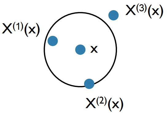
In more details, let $\left( X_{(i)}(x), Y_{(i)}(x) \right)$, $i=1..n$ denotes the $i$-th training data point closest to $x$ among all the training data points $\left( X_1, Y_1 \right)$, …, $\left( X_n, Y_n \right)$ such that the distance of each training data point to $x$ satisfies $d \left(x, X_{(1)}(x) \right)$ $\leq … \leq$ $d \left(x, X_{(n)}(x) \right)$.

By definition, the $k$-NN estimate for the label associated to $x$ is then⁹ the uniformly or non-uniformly weighted average label of the $k \in \{ 1,…,n \}$ nearest neighbors $Y_{(1)}(x)$,…,$Y_{(j)}(x)$

\[\hat{y} = \frac{1}{k} \sum_{i=1}^k Y_{(i)}(x)\]

or

\[\hat{y} = \sum_{i=1}^k w_i Y_{(i)}(x)\]

, where $w_i \geq 0$ is the weight associated to the $i$-th nearest neighbor $Y_{(i)}(x)$ and all the weights $w_i$, $i=1..k$ sum to one, that is, $\sum_{j=1}^k w_k$.

For illustration purposes, the process of selecting the 2 nearest neighbors $X_{(1)}(x)$ and $X_{(2)}(x)$ of a data point $x$ in $\mathbb{R}^2$ is outlined in Figure 2.

Figure 2. Example of $k$-NN nearest neighbors selection process in m = 2 dimensions, with n = 3 training data points and k = 2 nearest neighbors.

Notes:

• It additionally exists the $k$-NN classification algorithm, which is a variant of the $k$-NN regression algorithm where the label space is not $\mathbb{R}$ but a finite subset of $\mathbb{N}$.

Theoretical guarantees

Since the seminal paper of Cover and Hart¹⁰ - proving under mild conditions that the $k$-NN classification algorithm achieves an error rate that is at most twice the best error rate achievable⁸ -, several convergence results have been established for $k$-NN methods.

For example, under an asymptotic regime where the number of training data points $n$ and the number of nearest neighbors $k$ both go to infinity, it has been demonstrated⁹ that the $k$-NN regression algorithm is able to learn any functional relationship of the form $Y_i = f \left( X_i \right) + \epsilon_i$, $i=1..n$, where $f$ is an unknown function and $\epsilon_i$ represents additive noise.

As another example, this time under a finite¹¹ sample regime, Jiang¹² derives the first sup-norm finite-sample [“convergence”] result¹² for the $k$-NN regression algorithm and shows that it achieves a maximum error rate that is equal to the best maximum error rate achievable up to logarithmic factors¹², with high probability.

In addition to these convergence results, $k$-NN methods also exhibit interesting properties w.r.t. the dimensionality of the feature space $\mathbb{R}^m$.

For example, while the curse of dimensionality forces non-parametric methods such as $k$-NN to require an exponential-in-dimension sample complexity¹², the $k$-NN regression algorithm actually adapts to the local intrinsic dimension without any modifications to the procedure or data¹².

In other words, if the feature vectors belong to $\mathbb{R}^m$ but have a “true” dimensionality equal to $\mathbb{R}^p, p < m$, then the $k$-NN regression algorithm will [behave] as if it were in the lower dimensional space [of dimension $p$] and independent of the ambient dimension [$m$]¹².

Further properties of $k$-NN methods can be found in Chen and Shah⁸ and in Biau and Devroye⁹.

Practical performances

Like all supervised machine learning algorithms, the practical performances of the $k$-NN regression algorithm heavily depend on the problem at hand.

Yet, in general, it often yields competitive results [v.s. other more complex algorithms like neural networks], and in certain domains, when cleverly combined with prior knowledge, it has significantly advanced the state-of-the-art¹³.

Beyond these competitive performances, Chen and Shah⁸ also highlights other important practical aspects of $k$-NN methods that contributed to their empirical success over the years⁸:

• Their flexibility in choosing a problem-specific definition of “near” through a custom distance metric¹⁴
• Their computational efficiency, which has enabled these methods to scale to massive datasets (“big data”)⁸ thanks to approaches like approximate nearest neighbor search¹⁵ or random projections¹⁶
• Their non-parametric nature, in that they make very few assumptions on the underlying model for the data⁸
• Their ease of interpretability, since they provide evidence for their predictions by exhibiting the nearest neighbors found⁸

$k$-NN based supervised portfolios

Supervised portfolios

Chevalier et al.¹ describes an asset allocation strategy that engineers optimal weights before feeding them to a supervised learning algorithm¹, represented in the lower part of Figure 1.

Given a training dataset of past [financial] observations¹ like past asset returns, past macroeconomic indicators, etc., it proceeds as follows:

• For any relevant date¹⁷ $t=t_1,…$ in the training dataset

  • Compute optimal (in-sample) future portfolio weights $w_{t+1}$ over a (also in-sample) desired future horizon¹⁸, using a selected portfolio optimization algorithm with financial observations up to the time $t+1$

    These optimal future portfolio weights are the labels $Y_t$, $t=t_1,…$, of the training data points.

    To be noted that by lagging the data, we can use the in-sample future realized returns to compute all the [returns-based] estimates¹ required by the portfolio optimization algorithm like the expected asset returns, the asset covariance matrix, etc. This allows to be forward-looking in the training sample, while at the same time avoiding any look-ahead bias¹.

    During this step, constraints can of course be added in order to satisfy targets and policies¹.

  • Compute a chosen set of predictors supposed to be linked to the in-sample future portfolio weights $w_{t+1}$, using financial observations up to the time $t$

    These predictors are the feature vectors $X_t$, $t=t_1,…$, of the training data points.

• Train and tune a supervised machine learning algorithm using the training data points $\left( X_t, Y_t \right)$, $t=t_1,…$.

Once the training phase is completed, the supervised portfolio allocation algorithm is ready to be used with test data¹⁹.

• For any relevant (out-of-sample) test date $t’=t’_1,…$

  • Compute the set of predictors chosen during the training phase, using financial observations up to the time $t’$

    These predictors are the test feature vectors $x_{t’}$, $t’=t’_1,…$.

  • Provide that set of predictors as an input test feature vector to the supervised machine learning algorithm to receive in output the estimated optimal portfolio weights $\hat{w}_{t’+1}$ over the (out-of-sample) future horizon

    These estimated optimal portfolio weights are the estimated labels $\hat{y}_{t’}$, $t’=t’_1,…$.

    Here, depending on the exact supervised machine learning algorithm, the estimated portfolio weights $\hat{w}_{t’+1}$ might not satisfy the portfolio constraints²⁰ imposed in the training phase, in which case a post-processing phase would be required.

The portfolio allocation framework of Chevalier et al.¹ described above allows the algorithm to learn from past time series of in-sample optimal weights and to infer the best weights from variables such as past performance, risk, and proxies of the macro-economic outlook¹.

This contrasts with the standard practice of directly forecasting the input of a portfolio optimization algorithm, making that framework rather original.

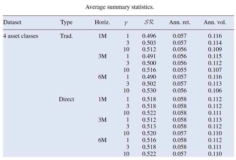
In terms of empirical performances, Chevalier et al.¹ finds that predicting the optimal weights directly instead of the traditional two step approach leads to more stable portfolios with statistically better risk-adjusted performance measures¹ when using mean-variance optimization as the selected portfolio optimization algorithm and gradient boosting decision trees as the selected supervised machine learning algorithm²¹.

Some of these risk-adjusted performance measures are displayed in Figure 3 in the case of 4 asset classes²², for the 3 horizons of predicted returns and the 3 risk aversion levels used in Chevalier et al.¹.

Figure 3. Performances of supervised portfolios v.s. direct mean-variance optimized portfolios, 4 asset classes. Source: Adapted from Chevalier et al.

Notes:

• Additional information can be found in the follow-up paper Chevalier et al.²³ and in a video of Thomas Raffinot for QuantMinds International.

$k$-NN-based supervised portfolios

Theoretically, the supervised machine learning model used in the portfolio allocation framework of Chevalier et al.¹ is trained to learn the following model¹:

\[w_{t+1} = g_t \left(X_t \right) + \epsilon_{t+1}\]

, where:

• $X_t $ is the feature vector made of the chosen set of predictors computed at time $t$
• $w_{t+1}$ is the vector of optimal portfolio weights over the desired future horizon $t+1$
• $g$ is an unknown function

Because such a model describes a functional relationship compatible with a $k$-NN regression algorithm, it is reasonable to think about using that algorithm as the supervised machine learning algorithm in the above framework.

Enter $k$-NN-based supervised portfolios, a portfolio allocation framework originally introduced in Varadi and Teed² as follows:

This naturally leads us down the path of creating algorithms that can learn from past data and evolve over time to change the method for creating portfolio allocations.

The simplest and most intuitive machine-learning algorithm is the K-Nearest Neighbor method ($k$-NN) […, which] is a form of “case-based” reasoning. That is, it learns from examples that are similar to current situation by looking at the past [and says: “what happened historically when I saw patterns that are close to the current pattern?”].

It shares a lot in common with how human beings make decisions. When portfolio managers talk about having 20 years of experience, they are really saying that they have a large inventory of past “case studies” in memory to make superior decisions about the current environment.

As a side note, Varadi and Teed² is not the first paper to apply a $k$-NN regression algorithm to the problem of portfolio allocation, c.f. for example Gyorfi and al.²⁴ in the setting of online portfolio selection, but Varadi and Teed² is - to my knowledge - the first paper about the same “kind” of supervised portfolios as in Chevalier et al.¹.

A couple of practical advantages of $k$-NN-based supervised portfolios v.s. for example “gradient boosting decision trees”-based supervised portfolios as used in Chevalier et al.¹ are:

• The simplicity of the training

  Since nearest neighbor methods are lazy learners, there is strictly speaking no real training phase.

• The simplicity of the tuning

  There can be no tuning at all if no “advanced” technique (automated features selection, distance learning…) is used.

• The guarantee that (convex) portfolio constraints learned during the training phase are satisfied during the test phase

  In $k$-NN regression²⁵, the estimate for the label associated to a test point is a convex combination of that point nearest neighbors.

  As a consequence, the estimated portfolio weights $\hat{w}_{t’+1}$ are guaranteed²⁵ to satisfy any learned convex portfolio constraints, thereby avoiding any post-processing that could degrade the “quality” of the estimated weights.

• The ease of interpretability

  Due to algorithm aversion, Chevalier et al.²³ highlights the need to be able to transform a black box nonlinear predictive algorithm [like gradient boosting decision trees] into a simple combination of rules²³ in order to make it interpretable for humans.

  With a $k$-NN regression algorithm, which is one of the most transparent supervised machine learning algorithm in existence, that step is probably not useful²⁶.

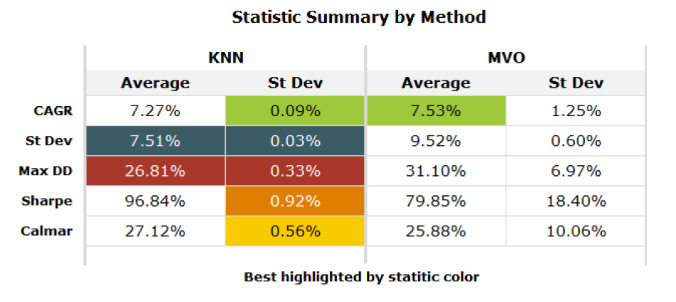
In terms of empirical performances, Varadi and Teed² concludes that $k$-NN-based supervised portfolios consistently outperformed [vanially maximum Sharpe ratio portfolios] on both heterogeneous and homogenous data sets on a risk-adjusted basis², with the $k$-NN-based approach [exhibiting] a Sharpe ratio [… up to] over 30% higher than [the direct maximum Sharpe ratio approach]².

Average performance measures for the $k$-NN-based supervised portfolios in Varadi and Teed² are reported in Figure 4.

Figure 4. Performances of $k$-NN-based supervised portfolios v.s. direct mean-variance optimized portfolios. Source: Adapted from Varadi and Teed.

Implementing $k$-NN-based supervised portfolios

Features selection

Biau and Devroye⁹ describes features selection as:

[…] the process of choosing relevant components of the [feature] vector $X$ for use in model construction.

There are many potential benefits of such an operation: facilitating data visualization and data understanding, reducing the measurement and storage requirements, decreasing training and utilization times, and defying the curse of dimensionality to improve prediction performance.

, and provides some rules of thumb that should be followed⁹:

• Noisy measurements, that is, components that are independent of $Y$, should be avoided⁹, especially because nearest neighbor methods are extremely sensitive to the features used²⁷
• Adding a component that is a function of other components is useless⁹

Beyond these generic rules, and although it has been an active research area in the statistics, machine learning, and data mining communities¹, features selection is unfortunately strongly problem-dependent.

In the context of supervised portfolios, Chevalier et al.¹ and Varadi and Teed² both propose to use:

• Past asset returns over different horizons²⁸ so as to assess momentum and reversals¹
• Past asset volatilities over different horizons²⁸, to approximate asset-specific risk¹

Varadi and Teed² additionally proposes to include past asset correlations over different horizons²⁸ to ensure that [the] $k$-NN algorithm [doesn’t] have access to any information that the [direct mean-variance optimization] [doesn’t] have, but merely use it differently².

Chevalier et al.¹, building on stocks asset pricing litterature, does not suggest to include other returns-based indicator than past asset returns and volatilities but suggests instead to include various macroeconomic indicators (yield curve, VIX…).

Features scaling

Typical distance metrics²⁹ used with nearest neighbor methods like the Euclidean distance are said to be scale variant, meaning that the definition of a nearest neighbor is influenced by the relative and absolute scale of the different features.

For example, when using the Euclidean distance with features such as a person’s height and a person’s age:

• The height feature disproportionally infuences the definition of a neighbor if the height feature is measured in millimeters and age in years
• The age feature disproportionally infuences the definition of a neighbor if the height feature is measured in meters and age in days

For this reason, features are usually scaled to a similar range before being provided in input to a $k$-NN algorithm³⁰, which is a pre-processing step called features scaling.

A couple of techniques for features scaling are described in Arora et al.³¹:

• Min-max scaling, which scales all the values of a feature $\left( X_i \right)_j$, $j \in \{ 1,…,m \}$, $i=1..n$ to a given interval - like $[0,1]$ -, based on the minimum and the maximum values of that feature:

  \[\left( X_i \right)_j' = \frac{\left( X_i \right)_j - \min_j \left( X_i \right)_j }{\max_j \left( X_i \right)_j - \min_j \left( X_i \right)_j }, i=1..n\]

• Standardization, also called z-score normalization, which transforms all the values of a feature $\left( X_i \right)_j$, $j \in \{ 1,…,m \}$ , $i=1..n$ into values that are approximatively standardly normally distributed:

  \[\left( X_i \right)_j' = \frac{ \left( X_i \right)_j - \overline{\left( X_i \right)_j}}{ \sigma_{\left( X_i \right)_j} }\]

In the context of supervised portfolios, additional techniques are described in Chevalier et al.¹:

• Quantile normal transformation for a “time series”-like feature, which standardizes the time-series into quantile and then map the values to a normal distribution¹

  It is important to note that at any given date, the quantiles should be computed using information up to that date only to avoid forward looking leakage¹.

  In addition, a lookback window over which to compute the quantiles should be chosen, with possible impacts on the performances of the supervised machine learning algorithm.

• Cross sectional normalization for a regular feature, which scales the cross sectional values between 0 and 1 using the empirical cumulative distribution function¹

  At any given date, this normalization can be performed fully in the cross-section at that date if there are enough assets or in the cross-section at that date using information up to that date to compute the empirical cumulative distribution function.

  In the latter case, c.f. the previous point.

• Hyperbolic tangent function ($\tanh$) scaling for labels, in order to center [them] and make them more comparable by taming outliers¹:

  \[Y' = 0.5 \tanh{\left( 0.01 \frac{Y − \overline{Y}}{ \sigma_Y } \right) }\]

  Naturally, the reverse transformation is performed after the prediction to transform back the labels into its original values¹.

Finally, in the specific context of $k$-NN-based supervised portfolios, 2 additional techniques are described in Varadi and Teed², that are variations of the techniques of Chevalier et al.¹.

Distance metric selection

As already mentioned in the previous sub-section, the distance metric used with a nearest neighbor method influences the definition of a nearest neighbor due to its scale variant or scale invariant nature.

But that’s not all, because different distance metrics behave differently with regards to outliers, to noise, to the dimension of the feature space, etc. On top of that, the chosen distance metric is sometimes not a proper metric⁶…

So, what to do in the specific context of $k$-NN-based supervised portfolios?

From the empirical results in Varadi and Teed², the Euclidean distance seems to be a good choice as long as the chosen predictors are properly scaled.

From the empirical results later in this blog post, a little known distance metric called the Hassanat distance³² also seems to be a good choice and additionally does not require³³ the chosen predictors to be scaled because it is scale invariant³⁴.

That distance - noted $HasD(x,y)$ - is defined between two vectors $x = \left(x_1,…,x_m\right)$ and $y = \left(y_1,…,y_m\right)$ as follows:

\[HasD(x,y) = \sum_{i=1}^m D(x_i,y_i)\]

, with

\[D(x_i,y_i) = \begin{cases} 1 - \frac{1 + \min(x_i,y_i)}{1 + max(x_i,y_i)}, &\text{if } \min(x_i,y_i) \geq 0 \\ 1 - \frac{1}{1 + \max(x_i,y_i) - min(x_i,y_i) } &\text{if } \min(x_i,y_i) < 0 \end{cases}\]

Figure 5 illustrates the 1-dimensional Hassanat distance $HasD(0,n)$ with $n \in [-10,10]$.

Figure 5. Representation of the 1-dimensional Hassanat distance between the points 0 and n. Source: Abu Alfeilat et al.

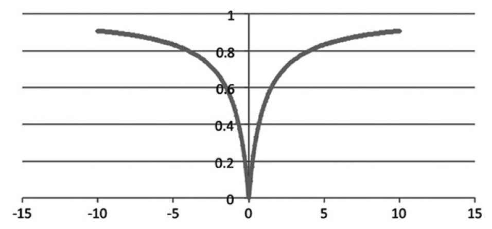
As a side note, the Hassanat distance has been empirically demonstrated to perform the best when applied on most data sets comparing with the other tested distances³⁵ in Abu Alfeilat et al.³⁵, which compares the performances of 54 distance metrics used in $k$-NN classification.

How to select the number of nearest neighbors?

Together with the distance metric $d$, the number of nearest neighbors $k$ is the other hyperparameter that has to be selected in nearest neighbor methods.

Varadi and Teed² explains:

The choice of the number of nearest matches (or neighbors) is the $k$ in $k$-NN.

This is an important variable that allows the benefit of allowing the use the ability to trade-off accuracy versus reliability. Choosing a value for $k$ that is too high will lead to matches that are not appropriate to the current case. Choosing a value that is too low will lead to exact matches but poor generalizability and high sensitivity to noise.

The optimal value for K that maximizes out-of-sample forecast accuracy will vary depending on the data and the features chosen.

In practice, the number of nearest neighbors $k$ […] [is] usually selected via cross-validation or more simply data splitting⁸ and the selected [value] minimizes an objective function which is often the Root Mean Square Error (RMSE) or sometimes the Mean Absolute Error (MAE)³⁶.

That being said, Guegan and Huck³⁶ cautions about that practice by highlighting that:

• The estimation of $k$ via in sample predictions leads to choose high values, near or on the border of one has tabulated because the RMSE is a decreasing function of the number of neighbors³⁶
• A high value for the number of nearest neighbors is an erroneous usage of the [method] because the neighbors are thus not near the pattern they should mimic³⁶, leading to (useless) forecasts very close to the mean of the sample³⁶.

Another direction is to adaptively choose the number of nearest neighbors $k$ […] depending on the test feature vector⁸.

For example, Anava and Levy³⁷ proposes solving an optimization problem to adaptively choose what $k$ to use for [a given feature vector] in an approach called $k^*$-NN⁸.

In the specific context of $k$-NN-based supervised portfolios, and again to avoid choosing an explicit number of nearest neighbors, Varadi and Teed² suggests to select a range³⁸ of $k$’s to make [the] selection base more robust to potential changes in an “optimal” $k$ selection².

Surprisingly, it turns out that this method is an ensemble method similar in spirit to the method described in Hassanat et al.³⁹ for $k$-NN classification, which consists in using a base $k$-NN classifier with $k=1,2,…,\lfloor \sqrt{n} \rfloor$ and to combine the $\lfloor \sqrt{n} \rfloor$ classification results using inverse logarithmic weights.

Misc. remarks

Importance of training dataset diversity

Asymptotic convergence results for the $k$-NN regression algorithm guarantee that by increasing the amount of [training] data, […] the error probability gets arbitrarily close to the optimum for every training sequence⁹.

But the amount of data available for training $k$-NN-based supervised portfolios is not infinite and might even in some cases be extremely limited⁴⁰.

In that case, there is a high risk that the training data is “unevenly balanced” in the feature space, a situation illustrated in Figure 6 in the case of a univariate feature whose underlying distribution is Gaussian.

Figure 6. Univariate $k$-NN regression with low accuracy, Gaussian feature distribution, far away training data. Source: Chen and Shah.

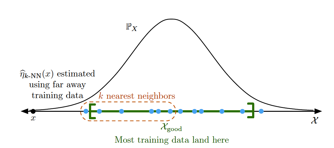
From Figure 6, it is clear that such a lack of training data - or more precisely, such a lack of diversity in the training data - would force the $k$-NN regression algorithm to use far away nearest neighbors, which would severely degrade the quality of the forecasted portfolio weights.

So, particular attention must be paid to the size and the diversity of the training dataset when using $k$-NN-based supervised portfolios, with for example ad-hoc procedures used whenever needed to simulate past asset returns for assets without return histories (here) or to extend return histories for assets with shorter return histories than others (here).

Avoiding the curse of dimensionality

The number of features selected by Varadi and Teed² grows quadratically with the number of assets.

At some point⁴¹, the underlying $k$-NN regression algorithm will then inevitably face issues due to:

• Distance concentration, which is the tendency of distances between all pairs of points in high-dimensional data to become almost equal⁴²
• Poor discrimination of the nearest and farthest points for a given test point, which is an issue on top of the distance concentration problem, c.f. Beyer et al.⁴³
• Hubness⁴², defined as the emergence of points called hubs which appear overly similar to many others
• …

In addition, the higher the number of features selected, the more training data is required to learn enough combinations of these different features, which further compounds the problem mentioned in the previous sub-section…

All in all, that approach is not scalable but hopefully, a solution is also proposed in Varadi and Teed²:

[…] to explore multi-asset portfolios [without introducing the problem of dimensionality with too-large a feature space], we took the average weight of each security from a single-pair run, and averaged them across all pair runs.

While this proposal may look like an ad-hoc workaround, it actually corresponds to an ensemble method that has been empirically shown to be effective for $k$-NN classification in high dimension in both:

• Domeniconi and Yan⁴⁴, with a deterministic selection of features as in Varadi and Teed²
• Bay⁴⁵, with a random²⁷ selection of features

The underlying idea of that ensemble method is to exploit [the] instability of $k$-NN classifiers with respect to different choices of features to generate an effective and diverse set of NN classifiers with possibly uncorrelated errors⁴⁴.

Implementations

Implementation in Portfolio Optimizer

Portfolio Optimizer supports $k$-NN-based supervised portfolios through the endpoint /portfolios/optimization/supervised/nearest-neighbors-based.

This endpoint supports 2 different distance metrics:

• The Euclidean distance matrix
• The Hassanat distance metric (default)

As for the selection of the number of nearest neighbors, this endpoint supports:

• A manually-defined number of nearest neighbors
• A dynamically-determined number of nearest neighbors together with their individual weights through:
  • The $k$-NN ensemble method of Hassanat et al.³⁹
  • A proprietary variation of the $k^*$-NN method of Anava and Levy³⁷ (default)

Implementation elsewhere

Chevalier et al.¹ kindly provides a Python code to experiment with “gradient boosting decision trees”-based supervised portfolios.

Example of usage - Learning maximum Sharpe ratio portfolios

Because most portfolio allocation decisions for active portfolio managers revolve around the optimal allocation between stocks and bonds², I propose to reproduce the results of Varadi and Teed² in the case of a 2-asset class portfolio made of:

• U.S. equities, represented by the SPY ETF
• U.S. long-term Treasury bonds, represented by the TLT ETF

Methodology

Varadi and Teed² follows the general procedure of Chevalier et al.¹ to train a $k$-NN-based supervised portfolio allocation algorithm for learning portfolio weights maximizing the Sharpe ratio.

For this, and without entering into the details:

• The selected features are asset returns, standard deviations and correlations over different²⁸ past lookback periods, scaled through a specific normal distribution standardization
• The selected distance metric is the standard Euclidean distance
• The selected number of nearest neighbors is not a single value but a range of values related to the size of the training dataset³⁸
• The relevant initial training dates are the 2000 daily dates present in Varadi and Teed²’s dataset from 4/13/1976 minus 2000 days to 4/12/1976

• The relevant subsequent training dates and test dates are all the daily dates present in Varadi and Teed²’s dataset from 4/13/1976 to 12/31/13

  To be noted that the training data is used in a rolling window manner over a 2000-day lookback.

• The future horizon over which maximum Sharpe ratio portfolio weights are learned during the training phase and evaluated during the test phase is a 20-day horizon

On my side:

• The selected features will be:
  • Past 12-month asset arithmetic returns, cross-sectionally normalized using the procedure described in Almgren and Neil⁴⁶
  • Future aggregated asset covariances forecasted over the next month using an exponentially weighted moving average covariance matrix forecasting model with daily squared (close-to-close) returns

• The selected distance metric will be the Hassanat distance

  This avoids the need for further features scaling.

• The selected number of nearest neighbors will be:
  • 1
  • 10
  • Dynamically determined with their individual weights by:
    • The $k$-NN ensemble method of Hassanat et al.³⁹
    • The $k^*$-NN method of Anava and Levy³⁷

• The relevant initial training dates will be all month-end dates present in a SPY/TLT ETFs-like training dataset from 1st January 1979 to 30 November 2003

  Due to the relatively recent inception dates of both the SPY ETF (22nd January 1993) and the TLT ETF (22th July 2002), it is required to use proxies to extend the returns history of these assets:

  • The daily U.S. market returns $Mkt$ provided in the Fama and French data library, as a proxy for the SPY ETF daily returns
  • The simulated daily returns associated to the daily FRED 30-Year Treasury Constant Maturity Rates, as a proxy for the TLT ETF daily returns

  With these, the earliest date for which daily SPY/TLT ETFs-like returns are available is 16th February 1977; adding 1 year of data for computing the past 12-month returns gives 16th February 1978; rounded to 1st January 1979.

• The relevant subsequent training dates and test dates will be all month-end dates present in the SPY/TLT ETFs test dataset from 1st January 2004 to 28th February 2025⁴⁷

  The earliest date for which daily SPY/TLT ETFs returns are available is 29th July 2002; adding 1 year of data for computing the past 12-month returns gives 29th July 2003; rounded to 1st January 2004.

  To be noted that the training data is used in an expanding window manner.

  As a consequence, the training dataset is made of 299 data points on 1st January 2004, expanding up to 552 data points on 28th February 2025 when the last forecast is made.

  This is in stark constrast with Varadi and Teed²’s training dataset which 1) contains 2000 data points and 2) is not expanding but is being rolled forward to keep the algorithm more robust to market changes in feature relevance².

  As mentionned in a previous section, such a difference in quantity and in “local” diversity of the training dataset might impact my results v.s. those of Varadi and Teed².

• The future horizon over which maximum Sharpe ratio portfolio weights are learned during the training phase and evaluated during the test phase is a 1-month horizon at daily level

• The risk free rate is set to 0% when computing maximum Sharpe ratio portfolio weights

• The cash portion of the different SPY/TLT portfolios - if any - is allocated to U.S. short-term Treasury bonds, represented by the SHY ETF

Results

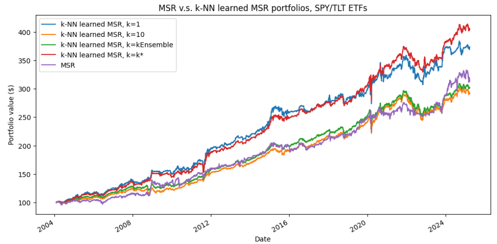
Figure 7 compares the standard direct approach for maximizing the Sharpe ratio to the $k$-NN-based supervised portfolios approach, with the 4 choices of nearest neighbors proposed in the previous sub-section.

In both cases, like in Varadi and Teed², the same features are used in input of the two algorithms.

Figure 7. MSR portfolio v.s. $k$-NN-based learned MSR portfolios, SPY/TLT ETFs, 1st January 2004 - 31th March 2025.

Summmary statistics:

Portfolio	CAGR	Average Exposure	Annualized Sharpe Ratio	Maximum (Monthly) Drawdown
Maximum Sharpe ratio (MSR)	~5.6%	~61%	~0.73	~14.4%
$k$-NN learned MSR, $k=1$	~6.4%	~49%	~0.86	~14.4%
$k$-NN learned MSR, $k=10$	~5.2%	~51%	~0.99	~15.8%
$k$-NN learned MSR, $k=kEnsemble$	~5.4%	~51%	~1.01	~15.1%
$k$-NN learned MSR, $k=k^*$	~6.8%	~49%	~1.00	~14.0%

Comments

A couple of comments are in order:

• Consistent with Varadi and Teed², the results demonstrate that the [$k$-NN-based supervised portfolio allocation] approach tends to outperform [the direct] MVO portfolio allocation [approach] on a risk-adjusted basis², with a Sharpe ratio ~18%-38% higher.

  This is quite interesting to highlight since the objective of the direct approach is supposed to be the maximization of the portfolio Sharpe ratio!

• The average exposure of the MSR portfolio is ~61% v.s. a relatively much lower exposure of ~50% for all the $k$-NN learned MSR portfolios

  The Sharpe ratio of all the $k$-NN learned MSR portfolios being higher than that of the MSR portfolio, it implies that the changes in exposure are pretty well “timed”.

• The $k$-NN learned MSR portfolios with $k=10$ and $k=kEnsemble$ are nearly identical

  This is confirmed by examining the underlying asset weights (not shown here).

  The $k$-NN ensemble portfolio has the advantage of not requiring to choose a specific value for $k$, though, and should definitely be prefered.

• The $k$-NN learned MSR portfolios with $k=1$ and $k=k^*$ are close in terms of raw performances, but not in terms of Sharpe ratio

  A closer look (not detailled here) reveals that this is because the $k$-NN learned MSR portfolios with $k=k^*$ regulary selects only 1 nearest neighbor when the other neighbors are too “far away” but also regularly selects many more neighbors when the other neighbors are “close enough”.

  I interpret this as an empirical demonstration of the ability of the $k^*$-NN method of Anava and Levy³⁷ to adaptively choose the number of nearest neighbors $k$ […] depending on the test feature vector⁸.

• The maximum drawdowns are comparable across all portfolios

  This shows that the $k$-NN learned MSR portfolios, despite their attractive risk-adjusted performancess, are not able to magically avoid “dramatic” events.

  Another layer of risk management, better return predictors, or both, is probably needed for that.

• The winner of this horse race is the $k$-NN learned MSR portfolios with $k=k^*$, but this comes at a price in terms of turnover v.s. the $k$-NN learned MSR portfolios with $k=kEnsemble$

  Also consistent with Varadi and Teed², the asset weights of the $k$-NN learned MSR portfolio with $k=kEnsemble$ (and with $k=10$) are relatively stable and on average similar to an equal weight portfolio, while those of the MSR portfolio show considerable noise and turnover².

  This is visible on the portfolio transition maps displayed in Figures 8 and 9.

  

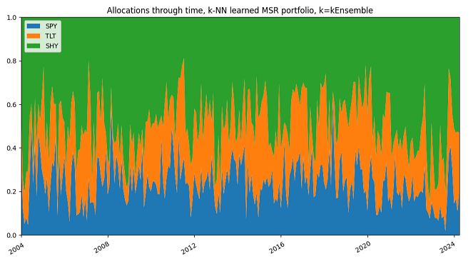
  Figure 8. $k$-NN-based learned MSR portfolio, $k=kEnsemble$, SPY/TLT/SHY ETFs allocations through time, 1st January 2004 - 31th March 2025.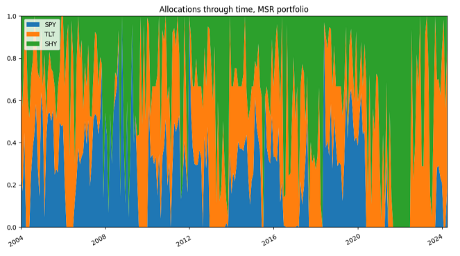

  

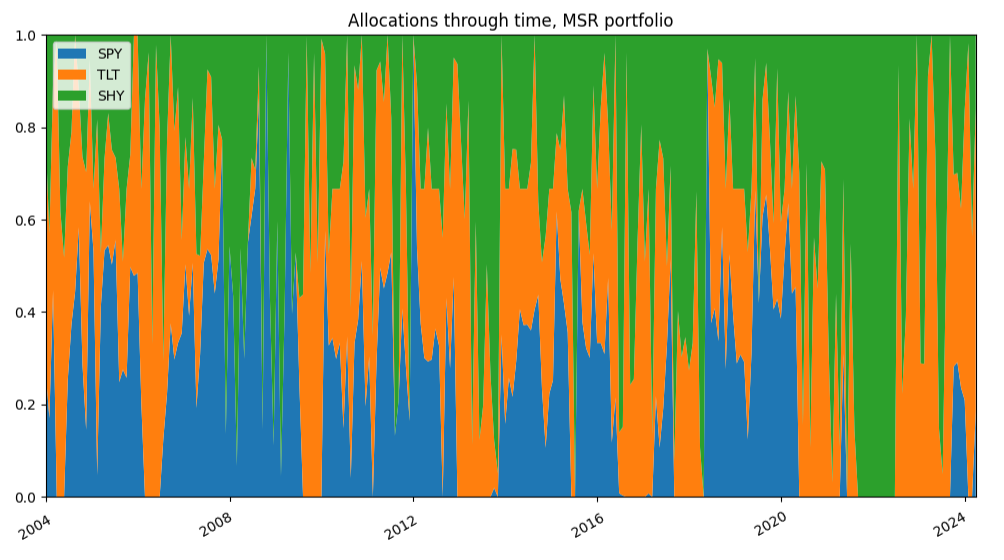
  Figure 9. MSR portfolio, SPY/TLT/SHY allocations through time, 1st January 2004 - 31th March 2025.

  For Varadi and Teed², this demonstrates the general uncertainty of the portfolio indicator inputs in aggregate² and that $k$-NN learned MSR portfolio with $k=kEnsemble$ manages to dynamically balance this uncertainty over time and shift more towards a probabilistic allocation that did not overweight or over-react to poor information².

  This statement is slightly less applicable to the $k$-NN learned MSR portfolio with $k=k^*$, because its better raw performances are explained by a more aggressive allocation, resulting in a much higher turnover, as can be seen by comparing Figure 8 to Figure 10.

  

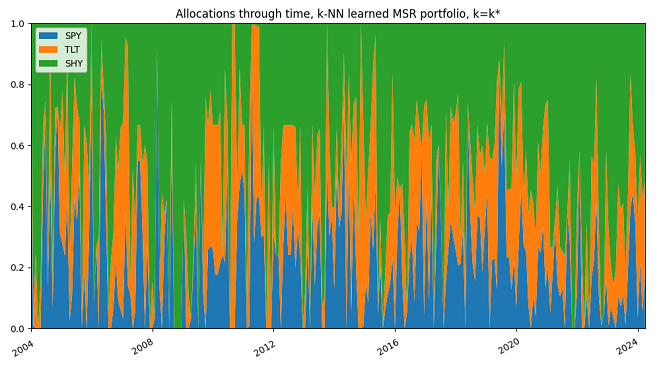
  Figure 10. $k$-NN-based learned MSR portfolio, $k=k^*$, SPY/TLT/SHY ETFs allocations through time, 1st January 2004 - 31th March 2025.

Conclusion

Exactly like in Varadi and Teed², and despite the differences in implementation and in the size of the training dataset⁴⁸:

• The results of this section shows that a traditional mean-variance/Markowitz/MPT framework under-performs [a $k$-NN-based supervised portfolio allocation] framework in terms of maximizing the Sharpe ratio²
• The data further implies that traditional MPT makes far too many trades and takes on too many extreme positions as a function of how it is supposed to generate portfolio weights²

Varadi and Teed² provides the following explanation:

This occurs because the inputs - especially the returns - are very noisy and may also demonstrate non-linear or counter-intuitive relationships. In contrast, by learning how the inputs map historically to optimal portfolios at the asset level, the resulting [$k$-NN-based supervised portfolios] allocations drift in a more stable manner over time.

Final conclusion

Supervised portfolios as introduced in Chevalier et al.¹ are able learn from past time series of in-sample optimal weights¹ and to infer the best weights from variables such as past performance, risk, and proxies of the macro-economic outlook¹.

In this blog post, I empirically demonstrated that this capability allows one of their simplest embodiement - $k$-NN-based supervised portfolios - to outperform a traditional mean-variance framework that seeks to maximize the Sharpe ratio of a portfolio, which independently confirms the prior results of Varadi and Teed².

To keep discovering non-standard portfolio allocation frameworks, feel free to connect with me on LinkedIn or to follow me on Twitter.

–

1. See Chevalier, G., Coqueret, G., & Raffinot, T. (2022). Supervised portfolios. Quantitative Finance, 22(12), 2275–2295. ↩ ↩² ↩³ ↩⁴ ↩⁵ ↩⁶ ↩⁷ ↩⁸ ↩⁹ ↩¹⁰ ↩¹¹ ↩¹² ↩¹³ ↩¹⁴ ↩¹⁵ ↩¹⁶ ↩¹⁷ ↩¹⁸ ↩¹⁹ ↩²⁰ ↩²¹ ↩²² ↩²³ ↩²⁴ ↩²⁵ ↩²⁶ ↩²⁷ ↩²⁸ ↩²⁹ ↩³⁰ ↩³¹ ↩³² ↩³³

2. See David Varadi, Jason Teed, Adaptive Portfolio Allocations, NAAIM paper. ↩ ↩² ↩³ ↩⁴ ↩⁵ ↩⁶ ↩⁷ ↩⁸ ↩⁹ ↩¹⁰ ↩¹¹ ↩¹² ↩¹³ ↩¹⁴ ↩¹⁵ ↩¹⁶ ↩¹⁷ ↩¹⁸ ↩¹⁹ ↩²⁰ ↩²¹ ↩²² ↩²³ ↩²⁴ ↩²⁵ ↩²⁶ ↩²⁷ ↩²⁸ ↩²⁹ ↩³⁰ ↩³¹ ↩³² ↩³³ ↩³⁴ ↩³⁵ ↩³⁶ ↩³⁷ ↩³⁸ ↩³⁹ ↩⁴⁰

3. Varadi and Teed² has been submitted to the 2014 NAAIM annual white paper competition known as the NAAIM Founders Award. ↩

4. To be noted that the data points could belong to a more generic space than $\mathbb{R}^m \times \mathbb{R}$. ↩

5. $\mathbb{R}^m$ is usually called the feature space. ↩

6. In practice, $d$ might not necessarily be a proper metric; for example, it might not satisfy the triangle inequality property like the cosine “distance”. ↩ ↩²

7. For an historical perspective on the $k$-NN algorithm going beyond the usual technical report from Fix and Hodges⁴⁹ and the seminal paper from Cover and Hart¹⁰, the interested reader is refered to Chen and Shah¹², which mentions that the $k$-NN classification algorithm was already mentioned in a text from the early 11th century. ↩

8. See George H. Chen; Devavrat Shah, Explaining the Success of Nearest Neighbor Methods in Prediction , now, 2018. ↩ ↩² ↩³ ↩⁴ ↩⁵ ↩⁶ ↩⁷ ↩⁸ ↩⁹ ↩¹⁰ ↩¹¹ ↩¹²

9. See Gerard Biau, Luc Devroye, Lectures on the Nearest Neighbor Method, Springer Series in the Data Sciences. ↩ ↩² ↩³ ↩⁴ ↩⁵ ↩⁶ ↩⁷ ↩⁸

10. See Cover, T. M. and P. E. Hart (1967). “Nearest neighbor pattern classification”. IEEE Transactions on Information Theory. ↩ ↩²

11. Although $n$ must be sufficiently large in order for there to exist a $k$ that satisfies the conditions¹² required by the main theorem of Jiang¹². ↩

12. See Jiang, H. (2019). Non-Asymptotic Uniform Rates of Consistency for $k$-NN Regression. Proceedings of the AAAI Conference on Artificial Intelligence, 33(01), 3999-4006. ↩ ↩² ↩³ ↩⁴ ↩⁵ ↩⁶ ↩⁷ ↩⁸ ↩⁹

13. See S. Sun and R. Huang, “An adaptive k-nearest neighbor algorithm,” 2010 Seventh International Conference on Fuzzy Systems and Knowledge Discovery, Yantai, China, 2010, pp. 91-94. ↩

14. See for example P.Y. Simard, Y. LeCun and J. Decker, “Efficient pattern recognition using a new transformation distance,” In Advances in Neural Information Processing Systems, vol. 6, 1993, pp. 50-58, in which the Euclidean distance between images of handwritten digits is replaced by an ad-hoc distance invariant with respect to geometric transformations of such images (rotation, translation, scaling, etc.). ↩

15. See Har-Peled, S., P. Indyk, and R. Motwani (2012). “Approximate Nearest eighbor: Towards Removing the Curse of Dimensionality.” Theory of Computing. ↩

16. See Kleinberg, J. M. (1997). “Two algorithms for nearest-neighbor search in high dimensions”. In: Symposium on Theory of Computing. ↩

17. For example, the end of each month for learning a monthly asset allocation strategy. ↩

18. A day, a week, a month, etc. ↩

19. Also called inference data, that is, data not “seen” during the training phase. ↩

20. Like budget constraints, asset weights constraints, asset group constraints, portfolio exposure constraints, etc. ↩

21. Chevalier et al.¹ notes that these empirical results still hold when replacing boosted trees by simple regressions¹. ↩

22. Developed equities, emerging equities, global corporate bonds, global government bonds. ↩

23. See Chevalier, Guillaume, Coqueret, Guillaume, Raffinot, Thomas, Interpretable Supervised Portfolios, The Journal of Financial Data Science Spring 2024, 6 (2) 10-34. ↩ ↩² ↩³

24. See L. Gyorfi, F. Udina, and H. Walk. Nonparametric nearest neighbor based empirical portfolio selection strategies. Statistics & Decisions, International Mathematical Journal for Stochastic Methods and Models, 26(2):145–157, 2008. ↩

25. Unless a very specific variation of $k$-NN regression is used. ↩ ↩²

26. At least from an algorithm aversion perspective. Nevertheless, there can be other benefits, c.f. Chevalier et al.²³. ↩

27. Similar to random subspace optimization. ↩ ↩²

28. 1 month, 2 months, 3 months, 6 months and 12 months. ↩ ↩² ↩³ ↩⁴

29. See Avivit Levy, B. Riva Shalom, Michal Chalamish, A Guide to Similarity Measures, arXiv for a very long list of distance metrics. ↩

30. Or more generally, to most supervised machine learning algorithms. ↩

31. See Ishan Arora and Namit Khanduja and Mayank Bansal, Effect of Distance Metric and Feature Scaling on KNN Algorithm while Classifying X-rays, RIF, 2022. ↩

32. See Hassanat, A.B., 2014. Dimensionality Invariant Similarity Measure. Journal of American Science, 10(8), pp.221-26. ↩

33. To be noted that features scaling might still be performed to try to improve the performances of the $k$-NN regression algorithm. ↩

34. Other properties of the Hassanat distance are for example robustness to noise and linear growth with the dimension of the feature space, c.f. Abu Alfeilat et al.³⁵. ↩

35. See Abu Alfeilat HA, Hassanat ABA, Lasassmeh O, Tarawneh AS, Alhasanat MB, Eyal Salman HS, Prasath VBS. Effects of Distance Measure Choice on K-Nearest Neighbor Classifier Performance: A Review. Big Data. 2019 Dec;7(4):221-248. ↩ ↩² ↩³

36. See Guegan, D. and Huck, N. (2005). On the Use of Nearest Neighbors in Finance. Finance, . 26(2), 67-86. ↩ ↩² ↩³ ↩⁴ ↩⁵

37. See Oren Anava, Kfir Levy, k*-Nearest Neighbors: From Global to Local, Advances in Neural Information Processing Systems 29 (NIPS 2016). ↩ ↩² ↩³ ↩⁴

38. In more details, Varadi and Teed² chooses the $k$’s in percentages of the size of the training space, which were 5%, 10%, 15% and 20% resulting essentially in a weighted average of the top instances². ↩ ↩²

39. See Hassanat, A.B., Mohammad Ali Abbadi, Ghada Awad Altarawneh, Ahmad Ali Alhasanat, 2014. Solving the Problem of the K Parameter in the KNN Classifier Using an Ensemble Learning Approach. International Journal of Computer Science and Information Security, 12(8), pp.33-39. ↩ ↩² ↩³

40. For example, due to the limited price history of some assets or due to the length of the desired horizon over which optimal portfolio weights need to be computed. ↩

41. Possibly for as few as 10-15 dimensions⁴³! ↩

42. See Radovanovic, Milo and Nanopoulos, Alexandros and Ivanovic, Mirjana}, Hubs in Space: Popular Nearest Neighbors in High-Dimensional Data, Journal of Machine Learning Research 11 (2010) 2487-2531. ↩ ↩²

43. See Beyer, K., Goldstein, J., Ramakrishnan, R., Shaft, U. (1999). When Is “Nearest Neighbor” Meaningful?. In: Beeri, C., Buneman, P. (eds) Database Theory — ICDT’99. ICDT 1999. Lecture Notes in Computer Science, vol 1540. Springer, Berlin, Heidelberg. ↩ ↩²

44. See Domeniconi, C., & Yan, B. (2004). Nearest neighbor ensemble. In Pattern recognition, international conference on, Vol. 1 (pp. 228–231). Los Alamitos, CA, USA: IEEE Computer Society. ↩ ↩²

45. See Bay S.D. Nearest neighbor classification from multiple feature subsets Intelligent Data Analysis, 3 (1999), pp. 191-209. ↩

46. See Almgren, Robert and Chriss, Neil A., Optimal Portfolios from Ordering Information (December 2004). ↩

47. (Adjusted) daily prices have have been retrieved using Tiingo. ↩

48. This empirically confirms that, desptite their dependency on the size of the training dataset, nearest neighbor methods can learn from a small set of examples⁴⁵. ↩

49. See Discriminatory analysis, nonparametric discrimination: Consistency properties”. Technical report, USAF School of Aviation Medicine. ↩