Sparse Index Tracking: Limiting the Number of Assets in an Index Tracking Portfolio

In the previous post, I introduced the index tracking problem¹, which consists in finding a portfolio that tracks as closely as possible² a given financial market index.

Because such a portfolio might contain any number of assets, with for example an S&P 500 tracking portfolio possibly containing ~500 stocks, it is [sometimes desirable] that the tracking portfolio consists of a small number of assets³ in order to simplify the execution, avoid small and illiquid positions, and large transaction costs³.

In other words, it is sometimes desirable to impose a constraint on the maximum number of assets contained in an index tracking portfolio, which leads to an extension of the regular index tracking problem called the sparse index tracking problem⁴.

In this new post, I will describe the mathematics of the sparse index tracking problem and I will detail a few examples of usage like:

• Replicating a fund of funds to reduce fees while keeping the number of directly-invested funds manageable
• Replicating the S&P 500 with only ~50 stocks as an (extreme) illustration of the optimized sampling⁵ ETF methodology

Mathematical preliminaries

The general sparse index tracking optimization problem

Let be:

• $T$, a number of time periods
• $r_{idx} = \left( r_{idx, 1}, …, r_{idx, T} \right) \in \mathcal{R}^{T}$, the vector of the index arithmetic returns over each of the $T$ time periods
• $n$, the number of assets in the universe of the sparse index tracking portfolio
• $X \in \mathcal{R}^{T \times n}$ the matrix of the $n$ assets arithmetic returns over each of the $T$ time periods
• $w = \left( w_1,…,w_n \right) \in \mathcal{R}^{n} $ the vector of the weights of a portfolio in each of the $n$ assets

The vector of the sparse index tracking portfolio weights $w^*$ is then the⁶ solution to the optimization problem which consists in minimizing a tracking error measure $f \left( X w - r_{idx} \right)$ - with $f$ some loss function - subject to additional constraints like full investment constraint, no short sale constraint, etc. and a cardinality constraint³

\[w^* = \operatorname{argmin} f \left( X w - r_{idx} \right) \newline \textrm{s.t. } \begin{cases} \sum_{i=1}^{n} w_i = 1 \newline 0 \leqslant w_i \leqslant 1, i = 1..n \newline ... \newline \lVert w \rVert_0 \le n_{max} \end{cases}\]

, where:

• $\lVert . \rVert_0$ is the zero “norm”⁷ of a vector, that is, the number of non-zero elements in that vector
• $n_{max}$ is the maximum number of assets with non-zero weights desired in the sparse index tracking portfolio

From a computational perspective, and whatever the exact definition of the loss function $f$, it is known that when a cardinality constraint restricting the number of stocks is introduced, the problem of optimizing the composition of a portfolio tends to become NP-hard⁸, which means that exact solutions to instances of realistic sizes are computationally intractable, and thus inexact solution methods are the only practical ones⁸.

Standard quadratic optimization methods guaranteeing an optimal solution are thus unfortunately not usable to solve the sparse index tracking optimization problem⁹…

Heuristics for solving the general sparse index tracking optimization problem

While an exhaustive enumeration of all possible methods for solving the sparse index tracking optimization problem is out of scope of this post, most of them¹⁰ seem to fall into one of three rough categories.

Combinatorial optimization methods

The cardinality constraint present in the sparse index tracking problem makes it a combinatorial problem, so that standard combinatorial optimization methods (continuous relaxation of a mixed integer programming formulation⁸¹¹, genetic algorithms¹²¹³…) can be used to find an approximate solution.

As a side note, thanks to the relationship of the sparse index tracking problem with combinatorial optimization and hence with operations research, it is possible to find datasets for different index tracking problems - ranging from a universe of 31 assets to a universe of 2151 assets - in the OR-Library.

Signal processing methods

The sparse index tracking problem in finance is closely related to a similar problem in signal processing called compressed sensing, for which specific algorithms have been developed over the years, like the iterative hard thresholding algorithm¹⁴ or the compressive sampling matching pursuit (CoSaMP) algorithm¹⁵.

To be noted, though, that all signal processing methods that rely on the least absolute shrinkage and selection operator (LASSO), which consists in approximating the $l_0$-norm constraint by a $l_1$-norm constraint, are not applicable to the sparse index tracking problem. Indeed, when full investment and no-short sales constraints are imposed¹⁶, we have, for any portfolio weights vector $w$

\[\lVert w \rVert_1 = \sum_{i=1}^n \left| w_i \right| = \sum_{i=1}^n w_i = 1\]

, so that the $l_1$-norm reduces to a constant and is therefore irrelevant³.

Non-linear optimization methods

At the crossroads with signal processing methods, generic non-linear optimization methods taking into account cardinality constraints have also been developed over the years:

• Methods that directly integrate cardinality constraints, like projected gradient methods¹⁷¹⁸ or coordinate descent methods¹⁸

• Methods that indirectly integrate cardinality constraints by either:

  • Relaxing the $l_0$-norm constraint into an “easier” constraint, like the entropic lower bound algorithm of Jacquet et al.¹⁹
  • Reformulating the $l_0$-norm constraint as a $l_0$-norm penalty integrated in the tracking error measure²⁰ and replacing that $l_0$-norm penalty with an “easier” penalty, like the $q$-norm approximation algorithm of Jansen and van Dijk²¹ or the majorization-minimization algorithm of Benidis et al.³

The sparse index tracking/empirical tracking error optimization problem

Like in the previous post of this series, this post will use the empirical tracking error as the preferred tracking error measure.

In this case, the general sparse index tracking optimization problem becomes

\[w^* = \operatorname{argmin} \frac{1}{T} \lVert X w - r_{idx} \rVert_2^2 \newline \textrm{s.t. } \begin{cases} \sum_{i=1}^{n} w_i = 1 \newline 0 \leqslant w_i \leqslant 1, i = 1..n \newline ... \newline \lVert w \rVert_0 \le n_{max} \end{cases}\]

, which, as noted by Benidis et al.³, is nothing else than a constrained sparse regression problem:

the sparse index tracking problem is similar to many sparsity formulations in the signal processing area in the sense that it is a regression problem with some sparsity requirements

Implementation in Portfolio Optimizer

Portfolio Optimizer allows to compute an approximate solution to the sparse index tracking optimization problem under the empirical tracking error measure through the endpoint /portfolios/replication/index-tracking/sparse.

In addition, Portfolio Optimizer allows to impose misc. constraints like minimum and maximum asset weights or minimum and maximum group weights constraints²².

Examples of usage

Replicating the S&P 500 by (extreme) optimized sampling

One of the most immediate application of the sparse index tracking problem is the ability to replicate a financial market index without investing into all its constituents, which is desirable for the reasons explained in the introduction of this post.

In order to illustrate this, I propose to partially replicate one of the numerical experiments in Benidis et al.³.

In details, using the S&P 500 data provided in the R package sparseIndexTracking - which consists in the daily returns of the S&P 500 index and of 386 of its constituents over the period from 1st January 2010 to 31th December 2010 - I will solve²³ the following 80 sparse index tracking problems:

• Index - S&P 500
• Tracking assets - 386 stocks included in the S&P 500
• Maximum number of assets - Varying from 20 to 100
• Misc. constraints - Maximum asset weight constraint of 5%

The empirical tracking error of the resulting 80 sparse S&P 500 tracking portfolios, as well as - for reference - the empirical tracking error of the regular S&P 500 tracking portfolio²⁴, is depicted in Figure 1.

Figure 1. Sparse S&P 500 tracking portfolios over the period 01 January 2010 - 31 December 2010, empirical tracking error v.s. maximum number of stocks

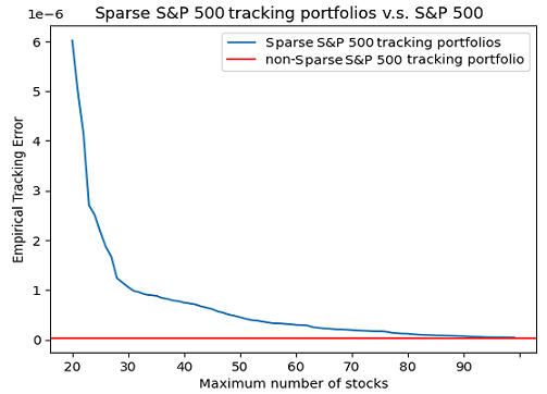
From this figure, it is visible that a sparse tracking portfolio made of ~100 stocks allows to track the S&P 500 with the same level of tracking error as a regular tracking portfolio made of much more stocks²⁴.

But it is possible to do better!

A sparse tracking portfolio made of only ~50 stocks is actually sufficient, as illustrated in Figure 2.

Figure 2. Sparse 55-stock S&P 500 tracking portfolio over the period 01 January 2010 - 31 December 2010, performances comparison with the S&P 500

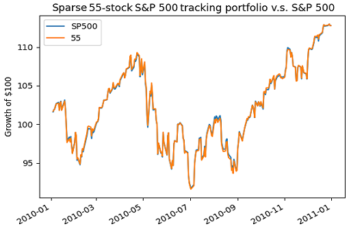
Of course, such a small portfolio might be less “diversified”²⁵ than its 100-stock counterpart, but the main takeaway is that a portfolio made of ~50-100 stocks adequately replicates the S&P 500, which opens the door of direct investing²⁶ to DIY investors.

Automatically determining the proper composite benchmark for a mutual fund

In the previous post of this series, the index tracking machinery was shown to allow to easily and automatically construct a benchmark for any mutual fund.

By extension, the sparse index tracking machinery also allows to do the same, with an important advantage for multi-asset mutual funds - the automated construction of the best composite benchmark with a given number of constituents.

Replicating a fund of funds to reduce fees

As a last example of usage, I propose to build upon a LinkedIn post from Finominal, in which the following question is asked:

What’s the likelihood that all […] funds in JP’s Investor Growth & Income Fund contribute value?

A bit of context first.

The JPMorgan Investor Growth & Income Fund is a fund of funds (FoF) whose main investment strategy is to invest in other J.P. Morgan Funds²⁷. As of 31 December 2023, it is invested in 25 such other J.P. Morgan funds (JPMorgan Core Bond R6, JPMorgan US Equity R6…).

One problem with FoF is that they usually have higher fees than traditional mutual funds because they include the management fees charged by the underlying funds²⁸.

The JPMorgan Investor Growth & Income Fund is no different, with a total expense ratio ranging from 1.47% to 0.72%, the latter being for its institutional class share (ticker ONGFX).

Inspired by the results from the previous post of this series, it is possible to reduce those fees by investing directly in all the underlying J.P. Morgan funds in proportion determined by solving²³ the following regular index tracking problem:

• Index - The JPMorgan Investor Growth & Income Fund (ONGFX)
• Tracking assets - 24 over the 25 J.P. Morgan funds held by the JPMorgan Investor Growth & Income Fund as of 31 December 2023, knowing that the 25th fund is marked as restricted for investment by Morningstar²⁹

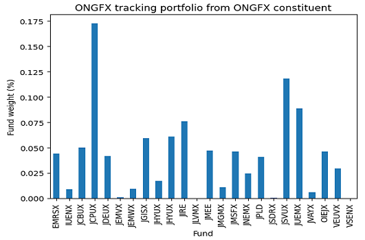
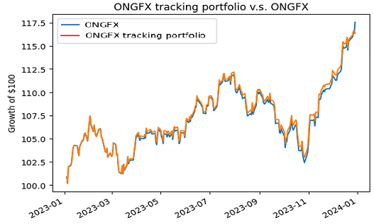
Using price data³⁰ for the period 01 January 2023 - 31 December 2023, this gives the regular tracking portfolio whose weights are displayed in Figure 3 and whose performances are compared with the JPMorgan Investor Growth & Income Fund in Figure 4.

Figure 3. JPMorgan Investor Growth & Income Fund tracking portfolio over the period 01 January 2023 - 31 December 2023, composition

Figure 4. JPMorgan Investor Growth & Income Fund tracking portfolio over the period 01 January 2023 - 31 December 2023, performances comparison with JPMorgan Investor Growth & Income Fund

This tracking portfolio has:

• A practically null tracking error v.s. the JPMorgan Investor Growth & Income Fund (Figure 4)
• An expense ratio of ~0.43%³¹ v.s. of at least 0.72% for the JPMorgan Investor Growth & Income Fund

So, this tracking portfolio is an interesting alternative to the JPMorgan Investor Growth & Income Fund, but there is a catch - it is invested in a total of 22 J.P. Morgan funds (Figure 3), which might be cumbersome to manage…

An even better tracking portfolio would have a smaller number of directly-invested funds.

Does such a unicorn exist?

Figures 5 and 6 answer this question, by solving²³ the following sequence of sparse index tracking problems over the period 01 January 2023 - 31 December 2023:

• Index - The JPMorgan Investor Growth & Income Fund (ONGFX)
• Tracking assets - The 24 non-restricted J.P. Morgan funds held by the JPMorgan Investor Growth & Income Fund as of 31 December 2023, knowing that the 25th fund is marked as restricted for investment by Morningstar²⁹
• Maximum number of assets - Varying from 1 to 24

Figure 5. Sparse JPMorgan Investor Growth & Income Fund tracking portfolio over the period 01 January 2023 - 31 December 2023, performances comparison with JPMorgan Investor Growth & Income Fund

Figure 6. Sparse JPMorgan Investor Growth & Income Fund tracking portfolio over the period 01 January 2023 - 31 December 2023, fees

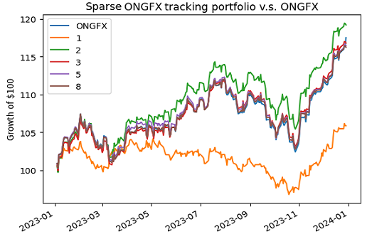
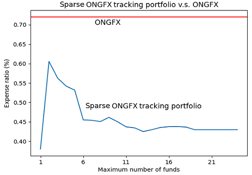
From these two figures, the sweet spot for the number of directly-invested funds in terms of tracking error/fees/manageability seems to be ~6-8.

Coming back to the initial question from Finominal, this analysis confirms that there is basically zero likelihood that all […] funds in JP’s Investor Growth & Income Fund contribute value, because these can be drastically reduced³².

Conclusion

That’s it for the first blog post of 2024!

Next in this series, I will discuss another extension of the regular index tracking problem, aiming this time at tracking a financial index with “dynamic” asset weights over the considered $T$ time periods.

As usual, feel free to connect with me on LinkedIn or to follow me on Twitter.

–

1. Also called the benchmark replication problem. ↩

2. In terms of a given tracking error measure, like the empirical tracking error³, also called the mean squared tracking error. ↩

3. See Konstantinos Benidis; Yiyong Feng; Daniel P. Palomar, Optimization Methods for Financial Index Tracking: From Theory to Practice , now, 2018.. ↩ ↩² ↩³ ↩⁴ ↩⁵ ↩⁶ ↩⁷ ↩⁸

4. Also called the partial benchmark replication problem. ↩

5. See Kees van Montfort, Elout Visser, Laurens Fijn van Draat, Index Tracking by Means of Optimized Sampling, The Journal of Portfolio Management Winter 2008, 34 (2) 143-152. ↩

6. Or a solution, in case multiple solutions exist. ↩

7. The zero “norm” is not a real norm. ↩

8. See Purity Mutunge, Dag Haugland, Minimizing the tracking error of cardinality constrained portfolios, Computers & Operations Research, Volume 90, 2018, Pages 33-41. ↩ ↩² ↩³

9. To be noted that in the specific case of a quadratic loss function, Mutunge and Haugland⁸ establish that the sparse index tracking optimization problem is actually strongly NP-hard. ↩

10. Excluding simple heuristics like selecting the largest assets according to a given criteria. For example, a widely used method, especially for a market capitalization weighted index, is to select the largest K assets according to their market capitalizations³; as another example, greedy or reverse greedy algorithms can be used on top of a non-sparse formulation of the index tracking problem to include or exclude assets one by one¹⁹. ↩

11. See N.A. Canakgoz, J.E. Beasley, Mixed-integer programming approaches for index tracking and enhanced indexation, European Journal of Operational Research, Volume 196, Issue 1, 2009, Pages 384-399. ↩

12. See J.E. Beasley, N. Meade, T.-J. Chang, An evolutionary heuristic for the index tracking problem, European Journal of Operational Research, Volume 148, Issue 3, 2003, Pages 621-643. ↩

13. See Gilli, M., Kellezi, E. (2002). The Threshold Accepting Heuristic for Index Tracking. In: Pardalos, P.M., Tsitsiringos, V.K. (eds) Financial Engineering, E-commerce and Supply Chain. Applied Optimization, vol 70. Springer, Boston, MA. ↩

14. See T. Blumensath and M. Davies, Iterative hard thresholding for compressed sensing, Appl. Comput. Harmon. Anal., 27 (2009), pp. 265–274.. ↩

15. See Deanna Needell and Joel A Tropp. Cosamp: iterative signal recovery from incomplete and inaccurate samples. Applied and Computational Harmonic Analysis, 26(3):301–321, 2009. ↩

16. Which is usually the case in practice… ↩

17. See Xu, F., Dai, Y., Zhao, Z. et al. Efficient projected gradient methods for cardinality constrained optimization. Sci. China Math. 62, 245–268 (2019).. ↩

18. See Amir Beck, Yonina C. Eldar, Sparsity Constrained Nonlinear Optimization: Optimality Conditions and Algorithms, 2013, SIAM Journal on Optimization, 1480-1509, 23, 3 ↩ ↩²

19. See Quentin Jacquet, Agnes Bialecki, Laurent El Ghaoui, Stéphane Gaubert, Riadh Zorgati. Entropic Lower Bound of Cardinality for Sparse Optimization. 2022.. ↩ ↩²

20. It is not trivial to show that such a reformulation is equivalent; c.f. Jansen and van Dijk²¹ for a detailed proof. ↩

21. See Roel Jansen, Ronald van Dijk, Optimal Benchmark Tracking with Small Portfolios, The Journal of Portfolio Management, Winter 2002, 28 (2) 33-39. ↩ ↩²

22. The possibility to include minimum and maximum group weights constraints is important in practice, because it allows for example to set an upper limit on fees or to (try to) impose sector neutrality in the computed portfolio, a characteristic often overlooked c.f. for example Che et al.³³ ↩

23. Using Portfolio Optimizer. ↩ ↩² ↩³

24. The non-sparse S&P 500 tracking portfolio, subject to the same maximum asset weight constraint of 5% as the sparse S&P 500 tracking portfolios, is made of 286 stocks. ↩ ↩²

25. For example, subject to sector concentration bias, as highlighted in Che et al.³³. ↩

26. Direct investing solutions are usually provided by asset management firms (Fidelity, Frec…). In the case of a stock market index, investing directly in stocks composing that stock market index, as opposed to indirectly through an ETF, has several advantages (null expense ratio, possibility to do tax-loss harvesting…). ↩

27. C.f. the JPMorgan Investor Growth & Income Fund prospectus. ↩

28. C.f. Wikipedia. ↩

29. C.f. Morningstar. ↩ ↩²

30. (Adjusted) prices have have been retrieved using Tiingo. ↩

31. Computation made using the expense ratios reported by Morningstar for the different J.P. Morgan funds, you will have to trust me on this one. To also be noted that the fees associated to the potential rebalancing of the tracking portfolio are not taken into account and would need to be properly minimized in real life. ↩

32. In view of Figure 5 and Figure 6, I would take the returns increased part of Finominal’s LinkedIn post with a grain of salt, although it is certain that returns will increase thanks to lowering the fees. ↩

33. See Che, Y.; Chen, S.; Liu, X. Sparse Index Tracking Portfolio with Sector Neutrality. Mathematics 2022, 10, 2645.. ↩ ↩²