Index Tracking: Reproducing the Performance of a Financial Market Index (and more)
An index tracking portfolio1 is a portfolio designed to track as closely2 as possible a financial market index when its exact replication3 is either impractical or impossible due to various reasons4 (transaction costs, liquidity issues, licensing requirements…).
In this blog post, after reviewing the underlying mathematics described in Hallerbach5, I will review a couple of applications of index tracking beyond “pure” index tracking, like helping financial advisors to reduce their customers investment fees or minimizing the sensitivity of mean-variance optimization to estimation error.
Notes:
- A Google Sheet corresponding to this post is available here
Mathematical preliminaries
The general index tracking optimization problem
Let be:
- $T$, a number of time periods
- $r_{idx} = \left( r_{idx, 1}, …, r_{idx, T} \right) \in \mathcal{R}^{T}$, the vector of the index arithmetic returns over each of the $T$ time periods
- $r_{tracking} = \left( r_{tracking, 1}, …, r_{tracking, T} \right) \in \mathcal{R}^{T}$, the vector of the (yet to be computed) index tracking portfolio arithmetic returns over each of the $T$ time periods
Then:
-
For a given time period $t$, the difference between the index return $r_{idx, t}$ and the index tracking portfolio return $r_{tracking, t}$ is defined as the tracking error $TE_t$:
\[TE_t = r_{tracking, t} - r_{idx, t}\] -
For all time periods $t=1..T$, the vector of the tracking errors $TE_t$ is defined as the tracking error vector $TE \in \mathcal{R}^{T}$:
\[TE = \left( r_{tracking, 1} - r_{idx, 1}, ..., r_{tracking, T} - r_{idx, T}\right)\]
Now, let be:
- $n$, the number of assets in the universe of the index tracking portfolio
- $w = \left( w_1,…,w_n \right) \in \mathcal{R}^{n} $ the vector of the weights of a portfolio in each of the $n$ assets
- $r_i = \left( r_{i, 1}, …, r_{i, T} \right) \in \mathcal{R}^{T}$, the vector of the asset $i$ arithmetic returns over each of the $T$ time periods, $i = 1..n$
Because arithmetic returns can be aggregated across assets, we have for each time period $t$:
\[r_{tracking, t} \left( w \right) = \sum_{i=1}^n w_i r_{i, t}\]So that:
\[TE_t \left( w \right) = \sum_{i=1}^n w_i r_{i, t} - r_{idx, t}\]and:
\[TE \left( w \right) = X w - r_{idx}\], with $X \in \mathcal{R}^{T \times n}$ the matrix of the $n$ assets arithmetic returns over each of the $T$ time periods.
The vector of the index tracking portfolio weights $w^$ is then the6 solution to the general index tracking optimization problem which consists in minimizing some loss function $f$ of the tracking error vector $TE$ - called *tracking error measure - subject to additional constraints like full investment constraint, no short sale constraint, etc.5
\[w^* = \operatorname{argmin} f(TE \left( w \right) ) \newline \textrm{s.t. } \begin{cases} \sum_{i=1}^{n} w_i = 1 \newline 0 \leqslant w_i \leqslant 1, i = 1..n \newline ... \end{cases}\]Tracking error measures
A common tracking error measure is the empirical tracking error (ETE)4, also called the mean squared tracking error (MSTE), defined as the sum of the squared tracking errors $TE_t$, $t=1..T$
\[ETE(w) = \frac{1}{T} \lVert X w - r_{idx} \rVert_2^2\]or, equivalently, the root mean square tracking error (RMSTE)5, defined by
\[RMSTE(w) = \sqrt{\frac{1}{T} \lVert X w - r_{idx} \rVert_2^2}\]Another common tracking error measure is the tracking error variance (TEV)5, defined as the variance of the tracking errors $TE_t$, $t=1..T$
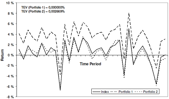
\[TEV(w) = Var( X w - r_b )\]However, as noted in Beasley et al.7, the usage of the tracking error variance is problematic due to its insensitivity to bias in the tracking errors $TE_t$. Indeed, if the index tracking portfolio returns $r_{tracking}$ are systematically higher or lower than the index returns $r_{idx}$8, the tracking error variance is null although the index tracking portfolio systematically deviates from its index!
This limitation is illustrated in Figure 1, adapted from Rossbach and Karlow9, in which it is clearly visible that portfolio 1 has a worse tracking quality than portfolio 2 but the TEV of portfolio 1 is equal to zero9.
In addition to the empirical tracking error and to the tracking error variance, other tracking error measures also exist like the mean absolute deviation of the tracking errors9, the correlation between the index tracking portfolio returns $r_{tracking}$ and the index returns $r_{idx}$5, the downside risk4, etc., but they will not be detailed in this blog post.
In all cases, it is important to note that different tracking error measures lead to different solutions to the general index tracking optimization problem - that is, different index tracking portfolios - with different properties10.
The index tracking/empirical tracking error optimization problem
Due to the limitation of the tracking error variance highlighted in the previous sub-section, this blog post will use the empirical tracking error as the preferred tracking error measure11.
In this case, the general index tracking optimization problem becomes a constrained regression problem in which the tracking errors $TE_t$, $t = 1..T$ represent the error terms:
\[w^* = \operatorname{argmin} \frac{1}{T} \lVert X w - r_{idx} \rVert_2^2 \newline \textrm{s.t. } \begin{cases} \sum_{i=1}^{n} w_i = 1 \newline 0 \leqslant w_i \leqslant 1, i = 1..n \newline ... \end{cases}\]From this perspective, and although index tracking is driven from the financial industry, it is in fact a pure signal processing problem4 that can be solved with standard quadratic optimization algorithms.
Caveats
The index tracking optimization problem as presented in the previous sub-sections relies on a couple of assumptions that are best to keep in mind:
-
The6 solution to the index tracking optimization problem is the portfolio with the lowest in-sample tracking error measure, while out-of-sample performances are ultimately what matters
Rossbach and Karlow9 study the stability of standard tracking error measures, including the empirical tracking error and the tracking error variance, and conclude that9
The results indicate a poor stability for every of the […] traditional measures. Furthermore, the relation to the ex post tracking quality is weak.
Nevertheless, this problem can be attenuated by regularly re-computing an index tracking portfolio thanks to a rolling window of recent past returns, c.f. Benidis4.
-
The6 solution to the index tracking optimization problem has fixed asset weights, while a certain level of drift is always present in practice
To make the underlying optimization problem tractable, the index tracking portfolio is supposed to be constantly rebalanced at each in-sample time period $t=1..T$.
This assumption is likely to be violated in practice, so that evaluating the ex-post impact of other rebalancing strategies (buy and hold, etc.) is important.
Relationship with Sharpe’s returns-based style analysis
Returns-based style analysis (RBSA) is a methodology initially introduced by Sharpe1213 to evaluate the composition of a mutual fund in absence of detailed holdings information.
In details, returns-based style analysis consists in determining the combination of major asset classes - represented by market indices - which most closely replicate the actual performances of a mutual fund over a given time period.
Unsurprisingly, the underlying mathematical formulation is actually equivalent to that of the index tracking/tracking error variance optimization problem13, with a specific vocabulary:
- The index tracking portfolio is called the mutual fund style benchmark
- The index tracking portfolio weights vector $w$ is called the mutual fund effective asset mix
- For a given time period $t$
- The index tracking portfolio return $r_{tracking, t}$ is interpreted as the mutual fund return attributable to style, that is, the mutual fund return originating from its passive exposure to the different asset classes
- The tracking error $TE_t$ is interpreted as the mutual fund return attributable to selection, that is, the mutual fund return originating from the skill of the portfolio manager(s)
Relationship with factor analysis
Sharpe13 highlights that returns-based style analysis is a specific type of factor analysis
An asset class factor model can be considered a special case of the generic type. In such a model each factor represents the return on an asset class, and the sensitivities ([beta_i] values) are required to sum to 1 (100%).
Similarly, from the previous sub-section, index tracking can also be considered as a member of the more general family of methods for portfolio factor analysis.
Implementation in Portfolio Optimizer
Portfolio Optimizer implements three functionalities related to index tracking as presented in the previous section:
- The computation of the empirical tracking error between a portfolio and an index, through the endpoint
/portfolios/analysis/empirical-tracking-error - The computation of the tracking error variance between a portfolio and an index, through the endpoint
/portfolios/analysis/tracking-error-variance - The computation of the index tracking portfolio solution to the index tracking optimization problem under the empirical tracking error measure, through the endpoint
/portfolios/replication/index-tracking
Examples of usage
Tracking an index when no ETF is available
I propose to illustrate the “vanilla” usage of an index tracking portfolio when no ETF associated to an index is available due to regulatory reasons.
For the context, residents of France have access to a tax-efficient investment wrapper called Plan d’Epargne en Actions (PEA).
A limitation of this investment wrapper, though, is that non-European financial assets cannot be sheltered under it - like global ETFs (MSCI World ETFs, etc.) - unless they have specifically been issued as PEA-compatible.
For example:
- Investing in an ETF tracking the MSCI World Index is allowed within a PEA thanks for example to the Lyxor PEA Monde (MSCI World) ETF Capi ETF14
- Similarly, investing in an ETF tracking the MSCI Emerging Markets (EM) Index is allowed within a PEA thanks for example to the Amundi PEA MSCI Emg EMEA ESG Lead UE Acc ETF15
- Yet, investing in an ETF tracking the MSCI All Country World (ACWI) Index is NOT allowed within a PEA, because no PEA-compatible ETF which tracks that index has been issued16
Now, for the sake of the exercise, let’s suppose a French DIY investor would like to track the MSCI ACWI Index within her PEA.
As mentioned above, this cannot be done directly since there is no PEA-compatible ETF which tracks this index.
Nevertheless, this can be done indirectly17 through an adequate combination of a PEA-compatible MSCI World ETF and a PEA-compatible MSCI EM ETF!
Indeed, Figure 2 compares the evolution, over the period 31 December 2019 - 30 September 2023, of:
- The PEA-incompatible Lyxor MSCI All Country World UCITS ETF - Acc18
- The PEA-compatible portfolio invested 86% in the Lyxor PEA Monde (MSCI World) ETF Capi ETF and 14% in the Amundi PEA MSCI Emg EMEA ESG Lead UE Acc ETF
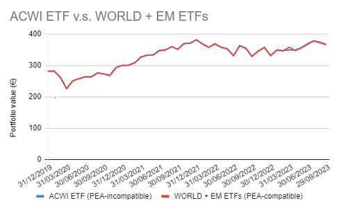
On this figure, it is visible that the tracking error between the two portfolios is almost null, which confirms that building a custom MSCI ACWI ETF inside a PEA is perfectly feasible19!
Question is, how have the weights of this PEA-compatible MSCI ACWI Index tracking portfolio been computed?
Well, it turns out that the problem at hand is an index tracking problem, with:
- Index - The PEA-incompatible Lyxor MSCI All Country World UCITS ETF - Acc18
- Tracking assets - The two PEA-compatible ETFs Lyxor PEA Monde (MSCI World) ETF Capi and Amundi PEA MSCI Emg EMEA ESG Lead UE Acc
Thus, using the monthly returns of these ETFs over the period 31 December 2019 - 30 September 2023, it is possible to compute the associated index tracking portfolio, which results in the PEA-compatible portfolio above.
Reducing the fees of a mutual funds portfolio
In the book Cloning Wall Street20, Jonathan Wallentine details how financial advisors can use index tracking portfolios - called replicating portfolios20 - to reduce portfolio fees for their clients.
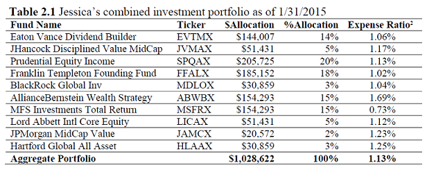
As an example from that book21, let’s suppose you are a financial advisor living in 2016 and a prospective client named Jessica comes to see you in order to decrease her mutual funds portfolio annual fees.
Jessica’s portfolio is made of the mutual funds listed22 in Figure 3, taken from Wallentine20.
After some thinking20, you conclude that Jessica’s mutual funds portfolio could probably be replaced by a portfolio made of the following low-cost ETFs:
- U.S. short term Treasuries (SHY ETF)
- U.S. aggregate bonds (AGG ETF)
- U.S. big caps stocks (SPY ETF)
- U.S. small caps stocks (IWM ETF)
- International stocks (EFA ETF)
Problem is, you don’t have a clue about the proportion to invest in each of these ETFs to properly replace Jessica’s portfolio…
What to do?
Here again, the problem at hand is actually an index tracking problem in disguise, with:
- Index - Jessica’s mutual funds portfolio
- Tracking assets - The five selected ETFs SHY, AGG, SPY, IWM and EFA
Thus, using the monthly returns of Jessica’s portfolio and of these five ETFs over the past period 2011 - 2015, it is possible to compute20 Jessica’s tracking portfolio weights:
- 5% in the SHY ETF
- 13% in the AGG ETF
- 54% in the SPY ETF
- 6% in the IWM ETF
- 22% in the EFA ETF
Figure 4, adapted from Wallentine20, depicts the evolution of Jessica’s original portfolio and of Jessica’s tracking portfolio.
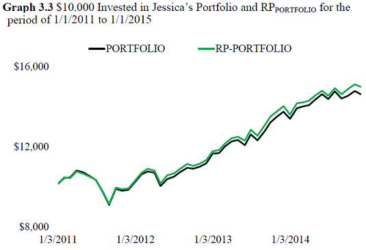
In addition to confirming a very small tacking error between the two portfolios, Figure 4 also highlights that Jessica’s tracking portfolio actually outperformed Jessica’s portfolio by 70bps annually2023.
Now, to come back on Jessica’s original request:
- Jessica’s mutual funds portfolio has an average expense ratio of 1.13%, which leads to total annual fees of around $11,62320
- Your alternative low-cost ETFs portfolio has an average expense ratio of 0.06%, which leads to total annual fees of around $61720
In other words, your alternative portfolio - which is for all intent and purposes equivalent to Jessica’s current portfolio - leads to a 95% decrease in annual fees24.
Jessica is delighted!
To conclude on this example, the results outlined in this [sub-]section should give readers confidence that [an index tracking portfolio] can successfully replicate a variety of different mutual fund portfolios from large fund companies20.
Automatically determining the proper benchmark for a mutual fund
In his 1992 paper, Sharpe notes that13
Style analysis provides a natural method for constructing benchmarks [for performance measurement]. The return obtained by a fund in each month can be compared with the return on a mix of asset classes with the same estimated style, where the style is estimated prior to the month in question.
Due to the one-to-one relationship between Sharpe’s style analysis and index tracking, the index tracking machinery then allows to easily and automatically construct a benchmark for any mutual fund25.
As an illustration, I propose to revisit a tweet from Nicolas Rabener - the founder and CEO of Finominal - in which an interesting discrepancy is reported between:
- The SEI Enhanced Low Volatility U.S. Large Cap (SELV) ETF
- The self-reported benchmark26 for this ETF - the Russell 1000 Index
For this, Figure 5 compares, over the period 01 January 2023 - 26 October 2023, the evolution of:
- The SELV ETF
- The iShares Russell 1000 (IWB) ETF, representative of the self-reported benchmark for the SELV ETF - the Russel 1000 Index
- The iShares MSCI USA Min Vol Factor (USMV) ETF, representative of the benchmark for the SELV ETF automatically determined by Finominal - the MSCI USA Minimum Volatility Index
- A portfolio made of 13% IWB ETF / 87% USMV ETF, representative of the benchmark for the SELV ETF automatically determined by Portfolio Optimizer using
- Index - The SELV ETF
- Tracking assets - The IWB and the USMV ETFs
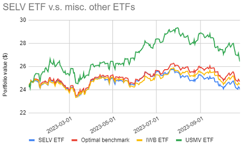
Figure 5 empirically demonstrates that the Russell 1000 Index is a very bad choice of benchmark for the SELV ETF and that a more realistic benchmark would consist either of:
- The MSCI USA Minimum Volatility Index, if only one index can be chosen
- The portfolio made of 13% Russel 1000 Index / 87% MSCI USA Minimum Volatility Index, if a composite index can be chosen27
These two alternative benchmarks are consistent with the SELV ETF fact sheet, which states that26
The SEI Enhanced Low Volatility U.S. Large Cap ETF seeks to provide long-term capital appreciation by investing primarily in U.S. common stocks, while aiming to experience lower volatility compared to the broad U.S. large cap equity market.
Coincidentally, Nicolas Rabener recently16 blogged about different metrics that can help selecting an optimal benchmark for a fund in his article Determining the Optimal Benchmark for Funds. Among these metrics, the tracking error is found to be the best performing one and results in nine selections [out of ten] that seem reasonable28.
As a side note, I wholeheartedly recommend readers interested in the topic of automatic benchmark selection to dig into the associated Finominal’s research blog posts.
Minimizing the sensitivity of mean-variance optimization to estimation error
A stylized fact of Markowitz’s mean-variance framework is the sensitivity of efficient portfolios to estimation error in asset returns and (co)variances29, which explains why efficient portfolios are sometimes labeled estimation-error maximizers30.
This issue is thoroughly analyzed, both theoretically and empirically, by Kinlaw et al.31 who conclude that
[mean-variance optimization] only appears to be hypersensitive when asset classes are close substitutes for each other, because the optimal weights may shift significantly in response to input errors.
In other words, Kinlaw et al.31 establish that it is possible to minimize the sensitivity of mean-variance optimization to estimation error by ensuring that assets are as “distinct” as possible.
A practical method for doing so is proposed in David Berns’ book Modern Asset Allocation for Wealth Management32.
In details, Berns’ methodology is a two-step procedure allowing to determine whether an asset in a portfolio is redundant with the other assets also present in that portfolio:
- Step 1 - Compute an index tracking portfolio - called the mimicking portfolio32 - using:
- Index - The selected asset
- Tracking assets - The other assets present in the portfolio
-
Step 2 - Assess the redundancy of the selected asset by looking at the tracking error [variance] between the mimicking portfolio and the asset32, because32
If the mimicking portfolio closely resembles [the selected] asset, then the [tracking error variance] will be low, and [the selected] asset is redundant and should be avoided to avoid estimation error sensitivity. However, if the [tracking error variance] for [the selected] asset is high, then [that] asset clearly showcases distinctness in one or more moments and can potentially be a valuable asset to consider for the portfolio.
In practice, Berns32 suggests to use a tracking error variance of around 2% as a reasonable level below which to start flagging assets for potential removal due to redundancy32.
Berns32 illustrates his proposed methodology using a portfolio made of intermediate-term Treasuries, intermediate-term investment grade bonds, and high-yield bonds. The mimicking portfolio for each asset is computed from the two other assets and the tracking error variance - called mimicking portfolio tracking error (MPTE) - between the mimicking portfolio and the asset under consideration is computed as in Figure 6, adapted from Berns32:
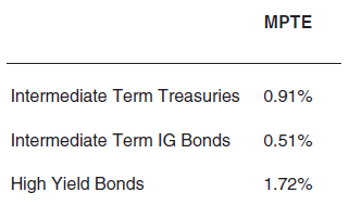
For this specific portfolio, intermediate-term investment grade bonds are flagged as the most redundant asset for reasons detailed in Berns32, but there is no real redundancy between the three assets33.
To be noted that other approaches for the problem of mean-variance optimization sensitivity to estimation error exist - like the computation of subset resampling-based efficient portfolios or the usage of the nested clustered optimization algorithm (NCO)34 - but these alternatives are usually much more mathematically involved than Berns’ modern yet practical32 approach.
Conclusion
Index tracking is a framework which deserves a place in one’s quantitative arsenal thanks to its versatility, as hopefully shown in this blog post.
Next in this series, I will discuss extensions of the basic index tracking problem, like for example methods to construct an index tracking portfolio with a limit on the number of assets it contains.
In the meantime, feel free to track me on LinkedIn or on Twitter.
–
-
Also called a benchmark replicating portfolio. ↩
-
The term closely is loosely defined at this point. ↩
-
From its constituent weights. ↩
-
See Konstantinos Benidis; Yiyong Feng; Daniel P. Palomar, Optimization Methods for Financial Index Tracking: From Theory to Practice , now, 2018.. ↩ ↩2 ↩3 ↩4 ↩5
-
See Hallerbach, W.G. (1994). Index Tracking: Some Techniques and Results. In: Peccati, L., Virén, M. (eds) Financial Modelling. Contributions to Management Science. Physica-Verlag HD. ↩ ↩2 ↩3 ↩4 ↩5
-
See J.E. Beasley, N. Meade, T.-J. Chang, An evolutionary heuristic for the index tracking problem, European Journal of Operational Research, Volume 148, Issue 3, 2003, Pages 621-643. ↩
-
That is, if $r_{tracking, t} = r_{idx, t} + c$, $t=1..T$, with $c$ a constant. ↩
-
See Rossbach, Peter and Karlow, Denis, (2011), The stability of traditional measures of index tracking quality, No 164, Frankfurt School - Working Paper Series, Frankfurt School of Finance and Management.. ↩ ↩2 ↩3 ↩4 ↩5
-
See Markus Rudolf, Hans-Jurgen Wolter, Heinz Zimmermann, A linear model for tracking error minimization, Journal of Banking & Finance, Volume 23, Issue 1, 1999, Pages 85-103. ↩
-
The empirical tracking error is not without issues, though; for example, it penalizes similarly both positive and negative deviations from the index. ↩
-
See Sharpe, William F, Determining a Fund’s Effective Asset Mix. Investment Management Review, December 1988, pp. 59-69. ↩
-
See William F. Sharpe, Asset allocation, Management style and performance measurement, The Journal of Portfolio Management, Winter 1992, 18 (2) 7-19. ↩ ↩2 ↩3 ↩4
-
FR0011869353 ↩
-
FR0011440478 ↩
-
At the date of the initial publication of this blog post. ↩ ↩2
-
The rationale is that by construction, all constituents of the MSCI ACWI Index belong either to the MSCI World Index or to the MSCI EM Index. ↩
-
Of course, this example of usage is very close to a toy example, but it already illustrates the potential of index tracking based on returns data. ↩
-
See Jonathan Wallentine, Cloning Wall Street, Actuarial Management Company. ↩ ↩2 ↩3 ↩4 ↩5 ↩6 ↩7 ↩8 ↩9 ↩10
-
Some of these mutual funds do not exist anymore at the date of publication of this post. ↩
-
As noted in Wallentine20, is likely the result of high mutual fund expense ratios in her portfolio (i.e. it is not due to any secret alpha generated by [the index tracking portfolio itself]20. ↩
-
One caveat, though, is that the index tracking portfolio needs to be purchased and then regularly re-balanced; also, as mentioned in Wallentine20, your management fees as advisor should of course be be taken into account. ↩
-
Or more generally, a benchmarka for any given asset. ↩
-
While not visible on Figure 5, the portfolio made of 13% IWB ETF / 87% USMV ETF has a lower empirical tracking error against the SELV ETF than the IWB ETF. ↩
-
See Broadie, M. Computing efficient frontiers using estimated parameters. Ann Oper Res 45, 21–58 (1993). ↩
-
See Michaud, Richard O., The Markowitz Optimization Enigma: Is ‘Optimized’ Optimal? (1989). Financial Analysts Journal, 1989. ↩
-
See William Kinlaw, Mark P. Kritzman, David Turkington, Asset Allocation: From Theory to Practice and Beyond, Wiley Finance. ↩ ↩2
-
See David M. Berns, Modern Asset Allocation for Wealth Management, Wiley Finance, 2020. ↩ ↩2 ↩3 ↩4 ↩5 ↩6 ↩7 ↩8 ↩9 ↩10
-
And no asset has a mimicking portfolio tracking error greater than 2%. ↩
-
See Lopez de Prado, Marcos, A Robust Estimator of the Efficient Frontier (October 15, 2016). ↩