Beyond Modified Value-at-Risk: Application of Gaussian Mixtures to the Computation of Value-at-Risk

In a previous post, I described a parametric approach to computing Value-at-Risk (VaR) - called modified VaR¹² - that adjusts Gaussian VaR for asymmetry and fat tails present in financial asset returns³ thanks to the usage of a Cornish–Fisher expansion.

Modified VaR, when properly used⁴, provides accurate estimates of the VaR for a wide range of non-normal portfolio return distributions. Unfortunately, for mathematical reasons, it cannot be computed for an even wider range of such distributions⁵, which poses an issue in practice.

In this blog post, I will describe another parametric approach to computing VaR - called Gaussian mixture Value-at-Risk for the lack of a better name - which this time adjusts Gaussian VaR for higher moments thanks to the usage of a Gaussian mixture distribution and is free of any computational restriction.

After providing the formula for the Gaussian mixture VaR and explaining how to fit a Gaussian mixture distribution to an empirical return distribution, I will show how to compute the Value-at-Risk of Bitcoin under the Gaussian mixture model described in the BlackRock paper Asset Allocation with Crypto: Application of Preferences for Positive Skewness from Ang et al.⁶

Mathematical preliminaries

Univariate Gaussian mixture distribution

A random variable $X$ is said to follow a univariate Gaussian mixture distribution, written as $X \sim \mathcal{GM} \left( \left( \mu_i, \sigma_i, p_i \right)_{i=1}^k \right) $, if its cumulative distribution function (c.d.f.) $F_X$ is of the form⁷

\[F_X(x) = \sum_{i=1}^k p_i \Phi \left( \frac{x - \mu_j}{\sigma_j} \right)\]

, where:

• $k \geq 1$ is the (integer) number of mixture components
• $p_i \in \left[ 0,1 \right]$, $i=1..k$, are the probabilities of the mixture components, with $\sum_{i=1}^kp_i = 1$
• $\mu_i \in \mathbb{R}$, $i=1..k$, are the means of the mixture components
• $\sigma_i \gt 0$, $i=1..k$, are the standard deviations of the mixture components
• $\Phi$ is the c.d.f. of the standard normal distribution

Reminder on Value-at-Risk

The (percentage) VaR of a portfolio of financial assets corresponds to the percentage of portfolio wealth that can be lost over a certain time horizon and with a certain probability.

Formally, the VaR $VaR_{\alpha}$ of a portfolio over a time horizon $T$ (1 day, 10 days…) and at a confidence level $\alpha$% $\in ]0,1[$ (95%, 97.5%, 99%…) can be defined as⁸

\[\text{VaR}_{\alpha} (X) = - F_X^{-1}(1 - \alpha)\]

, where:

• $X$ is a random variable representing the portfolio return over the time horizon $T$
• $F_X^{-1}$ is the inverse c.d.f. - also called the quantile function - of the random variable $X$

Gaussian mixture Value-at-Risk

Definition

When the return distribution of a portfolio is approximated by a Gaussian mixture distribution, that is, when $X \sim \mathcal{GM} \left( \left( \mu_i, \sigma_i, p_i \right)_{i=1}^k \right) $ with $X$ a random variable representing the portfolio return over a given time horizon $T$, the resulting parametric VaR can be called Gaussian mixture Value-at-Risk (GmVaR).

Mathematically, the Gaussian mixture VaR over the chosen time horizon $T$ and at a confidence level $\alpha$% $GmVaR_{\alpha}$ is implicitly defined by the following equation⁹, obtained by mixing together the formula for the VaR of a portfolio and the formula for the c.d.f. of a Gaussian mixture distribution

\[\sum_{i=1}^k p_i \Phi \left( - \frac{ GmVaR_{\alpha} + \mu_i }{\sigma_i} \right) = 1 - \alpha\]

Computation

Because the formula of the previous subsection is implicit in $GmVaR_{\alpha}$, the effective computation of the Gaussian mixture VaR must involve a numerical procedure such as:

• A non-linear least-squares minimization procedure⁹
• A bisection procedure¹⁰
• Or more generally, a procedure to compute a quantile function from a closed-form c.d.f.

Rationale

It has been observed since the 1970s¹¹ that Gaussian mixture distributions adequately approximate the unconditional distributions of financial asset returns. For example, Kon¹² shows that two, three and four-component Gaussian mixture distributions can be used to model the daily returns of 3 U.S. stock market indexes and of 30 Dow Jones stocks. Similarly, Cuevas-Covarrubias et al.¹³ shows how two-component Gaussian mixture distributions exhibit a natural capacity to fit leptokurtic distributions¹³ using the daily returns of 3 Mexican stocks.

Compared to alternative distributions, Gaussian mixture distributions offer a versatile combination of precision and simplicity¹³ for modeling asset returns. Indeed, Gaussian mixture distributions are both flexible enough to handle arbitrary asset return distributions¹⁴ and simple enough to be numerically tractable¹⁴. In contrast, [alternative distributions] tend to suffer from one of two evils: either they are too restrictive in the variety of p.d.f. shapes that can be achieved, or not restrictive enough, in the sense that they have too many degrees of freedom for calibration to be feasible¹⁴.

As for applications of Gaussian mixture distributions to VaR, Hull and White¹⁵ used a two-component Gaussian mixture distribution more than 25 years ago in order to illustrate their non-normal VaR computation methodology. More recent papers include for example Saissi Hassani and Dionne⁹ who performs VaR backtests for several parametric models, among which two and three-component Gaussian mixture models.

The Gaussian mixture VaR is thus a well-known extension of the Gaussian VaR when dealing with real-life asset returns.

Fitting a univariate Gaussian mixture distribution to an empirical portfolio return distribution

Let $r_1,…,r_T \in \mathbb{R}$ be the returns of a portfolio observed over $T$ time periods.

In order to compute the Gaussian mixture VaR of this portfolio using the formula of the previous section, it is first required to approximate the empirical distribution of the returns $r_1,…,r_T$ by a Gaussian mixture distribution.

This is usually done by determining the “best” statistical estimators for the unknown parameters $k$ and $\left(p_i, \mu_i, \sigma_i \right)$, $i=1..k$ of that Gaussian mixture distribution, with “best” to be defined.

How to determine the number of mixture components?

Manually

Because it is possible to interpret the components of a Gaussian mixture return distribution as market regimes, with a latent variable that represents the active regime and a return distribution that is Gaussian, given the regime⁷, the number of mixture components $k$ can be chosen manually.

For example:

• Choosing $k = 2$ means defining two market regimes in the portfolio returns - a normal regime and a rare events regime, sometimes called a distressed regime¹⁴ or a bliss regime⁶
• Choosing $k = 3$ means defining three market regimes in the portfolio returns - the typical bear, neutral and bull market regimes¹⁶

Automatically

The number of mixture components $k$ can also be chosen automatically through two general families of methods:

• Methods that determine the number of mixture components independently of the remaining mixture parameters

  Methods from this family typically iterate over a number of potential values for $k$, determine the remaining parameters $\left(p_i, \mu_i, \sigma_i \right)$, $i=1..k$, and evaluate how well the resulting $k$-component Gaussian mixture distribution approximates the portfolio return distribution.

  The chosen number of mixture components is then the value $k^*$, among these potential values for $k$, that allows to best approximate the portfolio return distribution¹⁷.

  Examples from this family include the Kolmogorov-Smirnov test¹⁸ or the more common Bayesian Information Criterion (BIC)¹⁹.

• Methods that determine the number of mixture components together with the remaining mixture parameters

  Methods from this family determine all the parameters of the Gaussian mixture distribution at once.

  Examples from this family include modified Expectation-Maximization algorithms²⁰ or ad-hoc procedures²¹.

How to determine the remaining mixture parameters?

In this subsection, the number of mixture components $k$ is supposed to be known²².

Likelihood maximization

Sensible values for the unknown mixture parameters $\left(p_i, \mu_i, \sigma_i \right)$, $i=1..k$, are maximum-likelihood estimates, defined as the choice of parameters $\left(p_i^*, \mu_i^*, \sigma_i^* \right)$, $i=1..k$, that globally²³ maximizes the log-likelihood function $L$ associated to the returns $r_1,…,r_T$ and given by

\[L \left( p_1, \mu_1, \sigma_1,..., p_k, \mu_k, \sigma_k \right) = \sum_{i=1}^T \ln \left[ \sum_{j=1}^k p_j \frac{1}{\sqrt{2 \pi} \sigma_j} \exp \left( - \frac{1}{2} \left( \frac{ x_i - \mu_j}{ \sigma_j} \right )^2 \right) \right]\]

Numerically, several procedures can be used to compute these maximum-likelihood estimates, like Newton’s method²⁴, Fisher’s method of scoring²⁴ or the Expectation-Maximization (EM) algorithm¹⁹ which is actually the method of choice for learning mixtures of Gaussians²⁵²⁶.

Unfortunately, due to the complexity²⁷ of the log-likelihood function $L$, none of these procedures is guaranteed to produce “true” maximum-likelihood estimates²⁸. Even worse, the behavior of all these procedures is known to be highly dependent from [the initial guess of the unknown parameters] and it may fail as a result of degeneracies²⁸, which led practitioners to implement misc. numerical tweaks, like running these procedures several times with different, randomly chosen starting points²⁹, in order to avoid [obtaining] a poor approximation to the true maximum²⁹.

Turbulence partitioning of returns

Although in most applications, parameters of a [Gaussian] mixture model are estimated by maximizing the likelihood²⁹, there are other procedures to determine the remaining parameters of a Gaussian mixture distribution (minimum distance estimation³⁰…) which have often been show to be more robust to departures from underlying assumptions than is maximum likelihood³⁰.

While an exhaustive review of these alternative procedures is out of scope of this post, I would still like to mention a procedure described in another post in the the context of a two-component Gaussian mixture distribution.

This procedure is based on a measure of statistical unusualness of asset returns popularized by Kritzman and Li³¹ called the Turbulence Index, and can easily be generalized to a $k$-component Gaussian mixture distribution as follows:

• Compute the turbulence index values $d(r_t)$, $t=1..T$, associated to the portfolio returns³²
• Partition the portfolio returns into $k$ partitions based on their turbulence index values, either through manual percentage-based thresholding³³ or through automated clustering (1D $k$-means³⁴…).
• For each of these partitions $P_i$,$i=1..k$
  • Define the estimate of the $i$-th Gaussian mixture component probability $p_i^{**}$ as the proportion of the portfolio returns belonging to $P_i$
  • Define the estimate of the $i$-th Gaussian mixture component mean $\mu_i^{**}$ as the mean of the portfolio returns belonging to $P_i$
  • Define the estimate of the $i$-th Gaussian mixture component standard deviation $\sigma_i^{**}$ as the standard deviation of the portfolio returns belonging to $P_i$

Compared to likelihood maximization, this procedure is:

• Easy to implement, with no local optima and no convergence issue to worry about
• Easy to interpret, with a one-to-one relationship between partitions and market regimes

In addition, as illustrated in the aforementioned post, the quality of the resulting parameters estimates is on par with that of the maximum-likelihood parameters estimates, at least in the case of a two-asset universe made of U.S. stocks and U.S. Treasuries.

Implementation in Portfolio Optimizer

Portfolio Optimizer implements the computation of a portfolio Gaussian mixture Value-at-Risk through the endpoint /portfolios/analysis/value-at-risk/gaussian/mixture.

This endpoint:

• Fits a univariate Gaussian mixture distribution to an empirical portfolio (logarithmic) return distribution, using either
  • A variation of the Expectation-Maximization algorithm described in the previous section
  • The turbulence partitioning procedure also described in the previous section, relying on either a percentage-based thresholding of turbulence index values or a 1D $k$-means clustering of turbulence index values
• Computes the associated Gaussian mixture Value-at-Risk, using a variation of the bisection procedure

To be noted that it is possible to let Portfolio Optimizer automatically determine the best number of Gaussian mixture components³⁵.

Example of usage - Computing the Value-at-Risk of Bitcoin

In their paper, Ang et al.⁶ empirically demonstrate that the very positively skewed returns [of Bitcoin] are well captured by a [two-component] mixture of Normals distribution⁶. They then use this result to suggest that given a small probability regime where Bitcoin may generate high returns, investors with preferences for positive skewness of portfolio returns should have portfolio exposure to Bitcoin³⁶.

As an example of usage of the Gaussian mixture VaR, I propose to compute the VaR of Bitcoin under such a two-component Gaussian mixture model.

Bitcoin returns analysis

I propose to start by comparing the Bitcoin price data used in Ang et al.⁶ to the Bitcoin price data used in this post:

• Figures 1³⁷ and 2 compare the cumulative returns of Bitcoin over the period 31 August 2010 - 31 December 2021

  

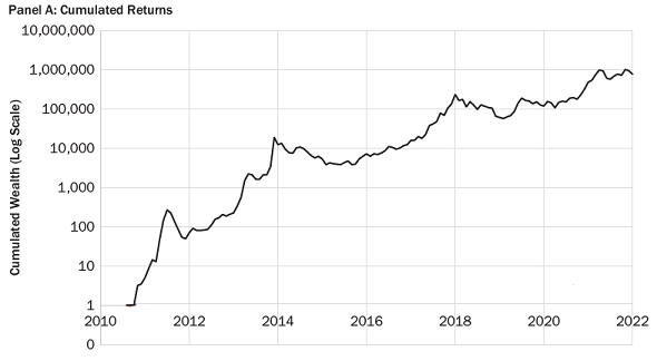
  Figure 1. Cumulative Bitcoin returns over the period 31 August 2010 - 31 December 2021, Ang et al.'s data. Source: Ang et al.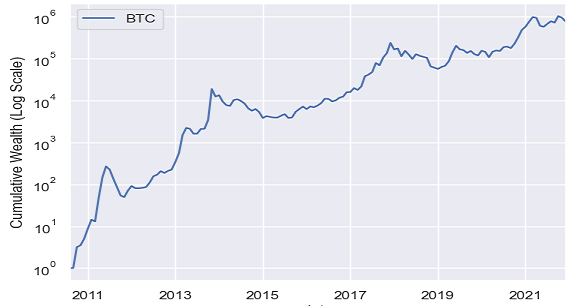

  

  Figure 2. Cumulative Bitcoin returns over the period 31 August 2010 - 31 December 2021, this post's data.

• Figures 3³⁷ and 4 compare the annualized mean, standard deviation and Sharpe ratio of Bitcoin monthly (log) returns over the same period

  

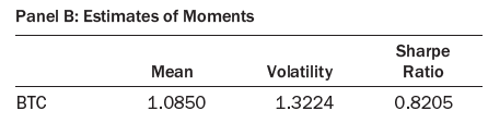
  Figure 3. Summary statistics of Bitcoin monthly returns over the period 31 August 2010 - 31 December 2021, Ang et al.'s data. Source: Ang et al.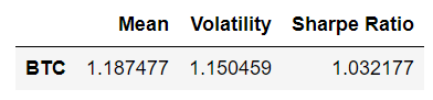

  

  Figure 4. Summary statistics of Bitcoin monthly returns over the period 31 August 2010 - 31 December 2021, this post's data.

From these figures, it is clear that the Bitcoin data used in Ang et al.⁶ differ from the Bitcoin data used in this post (Figure 3 v.s. Figure 4), although not that much (Figure 1 v.s. Figure 2).

To be noted that this is not surprising, because there is no official price for Bitcoin due to its decentralized nature.

Fitting a Gaussian mixture model to Bitcoin returns

Similar to Ang et al.⁶, I now propose to fit a two-component Gaussian mixture model to the Bitcoin monthly (log) returns over the period 31 August 2010 - 31 December 2021.

Likelihood maximization

The EM algorithm, as implemented by the scikit-learn method sklearn.mixture.GaussianMixture with default parameters, leads to three different maximum likelihood estimates³⁸

• $\left(p_1^1, \mu_1^1, \sigma_1^1 \right)$ = $\left( 0.96, 0.66, 0.84 \right)$ and $\left(p_2^1, \mu_2^1, \sigma_2^1 \right)$ = $\left( 0.04, 14.98, 0.89 \right)$
• $\left(p_1^2, \mu_1^2, \sigma_1^2 \right)$ = $\left( 0.91, 0.54, 0.82 \right)$ and $\left(p_2^2, \mu_2^2, \sigma_2^2 \right)$ = $\left( 0.09, 7.45, 2.03 \right)$
• $\left(p_1^3, \mu_1^3, \sigma_1^3 \right)$ = $\left( 0.91, 0.55, 0.82 \right)$ and $\left(p_2^3, \mu_2^3, \sigma_2^3 \right)$ = $\left( 0.09, 7.81, 2.03 \right)$

This situation confirms that an important drawback of EM is that its solution can highly depend on its starting position and consequently produce sub-optimal maximum likelihood estimates²⁹!

Fortunately, increasing the number of random initializations performed in the sklearn.mixture.GaussianMixture method leads to the optimal maximum likelihood estimates, but somebody unaware of the numerical properties of the EM algorithm might conclude too quickly that the mixture of Normals can be estimated easily by maximum likelihood or EM algorithms⁶.

These “true” maximum likelihood estimates are $ \left(p_1^*, \mu_1^*, \sigma_1^* \right)$ = $\left( 0.96, 0.66, 0.84 \right)$ and $\left(p_2^*, \mu_2^*, \sigma_2^* \right)$ = $\left( 0.04, 14.98, 0.89 \right)$.

Turbulence partitioning

The turbulence partitioning procedure used with an exact 1D $k$-means clustering leads to the same³⁹ estimates as the “true” maximum likelihood estimates, which empirically demonstrates the validity of this procedure to fit the parameters of a univariate Gaussian mixture distribution.

As a reminder, these estimates are $ \left(p_1^{**}, \mu_1^{**}, \sigma_1^{**} \right)$ = $\left( 0.96, 0.66, 0.84 \right)$ and $\left(p_2^{**}, \mu_2^{**}, \sigma_2^{**} \right)$ = $\left( 0.04, 14.98, 0.89 \right)$.

One of the advantages of the turbulence partitioning procedure is that it allows to easily explain how the Gaussian mixture parameters have been estimated:

• $p_1^{**}$ (resp. $p_2^{**}$) is the proportion of Bitcoin returns whose turbulence index values are classified as “normal” (resp. “outliers”) by the 1D $k$-means clustering method

  Graphically, thanks to Figure 5 which displays the 137 turbulence index values associated to the Bitcoin monthly (log) returns over the period 31 August 2010 - 31 December 2021:

  • $p_1^{**}$ is the proportion of Bitcoin returns whose turbulence index values are below the red horizontal line, that is, $p_1^{**} = \frac{132}{137} \approx 0.96$

  • $p_2^{**}$ is the proportion of Bitcoin returns whose turbulence index values are above the red horizontal line, that is, $p_2^{**} = \frac{5}{137} \approx 0.04$

  

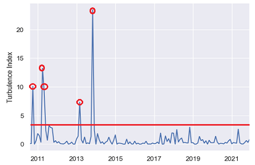
  Figure 5. Bitcoin monthly turbulence index values, 31 August 2010 - 31 December 2021.

• $\mu_1^{**}$ (resp. $\mu_2^{**}$) is the mean of the Bitcoin returns whose turbulence index values are classified as “normal” (resp. “outliers”) by the 1D $k$-means clustering method

• $\sigma_1^{**}$ (resp. $\sigma_2^{**}$) is the standard deviation of the Bitcoin returns whose turbulence index values are classified as “normal” (resp. “outliers”) by the 1D $k$-means clustering method

In terms of market regimes, the first (resp. second) Gaussian mixture component models the behavior of Bitcoin during a normal (resp. rare events) market regime.

As a side note, the turbulence partitioning procedure highlights that only 5 returns have been used to compute the parameters estimates $\left(p_2^{**}, \mu_2^{**}, \sigma_2^{**} \right)$, which raises the question of the statistical significance of both these estimates⁴⁰ and the maximum likelihood estimates $\left(p_2^*, \mu_2^*, \sigma_2^* \right)$ since they are equal…

Evaluation

Figure 6 and Figure 7 compare the theoretical distribution of the estimated two-component Gaussian mixture distribution with the empirical distribution of the monthly (log) Bitcoin returns.

Figure 6. Bitcoin monthly returns, empirical c.d.f. v.s. two-component Gaussian mixture c.d.f., 31 August 2010 - 31 December 2021.

Figure 7. Bitcoin monthly returns, empirical c.d.f. v.s. two-component Gaussian mixture c.d.f., left tail, 31 August 2010 - 31 December 2021.

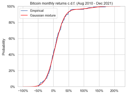
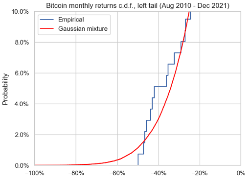
From these figures, the estimated mixture model seems to adequately capture the main characteristics of the Bitcoin returns, except part of their left tail behavior, which is confirmed more quantitatively by the Kolmogorov-Smirnov goodness of fit test⁴¹.

Bitcoin returns Value-at-Risk

I finally propose to compute the Value-at-Risk of Bitcoin monthly (log) returns over the period 31 August 2010 - 31 December 2021, using two methods:

• The historical Value-at-Risk (HVaR), introduced in another post
• The Gaussian mixture Value-at-Risk, introduced in this blog post

Results for various confidence levels, all visible on Figure 7, are provided below:

Confidence level $\alpha$	$\text{HVaR}_{\alpha}$	$\text{GmVaR}_{\alpha}$
95%	42.02%	34.21%
97.5%	45.84%	41.97%
99%	47.22%	50.96%
99.5%	49.86%	57.08%
99.9%	49.86%	69.69%

Conclusion

Aim of this post was to describe an extension of Gaussian Value-at-Risk, second in order of complexity after modified Value-At-Risk, in case the later cannot be computed.

This being done, I wish you Season’s Greetings and a Happy New Year!

Waiting for 2024, feel free to connect with me on LinkedIn or follow me on Twitter.

–

1. See Zangari, P. (1996). A VaR methodology for portfolios that include options. RiskMetrics Monitor First Quarter, 4–12. ↩

2. Or Cornish-Fisher VaR. ↩

3. In this post, all returns are assumed to be logarithmic returns. ↩

4. See Maillard, Didier, A User’s Guide to the Cornish Fisher Expansion. ↩

5. All portfolio return distribution for which the skewness and the (excess) kurtosis are outside of the domain of validity of the Cornish-Fisher expansion underlying modified VaR, c.f. Maillard⁴. ↩

6. See Ang, Andrew, Morris, Tom, Savi, Raffaele, Asset Allocation with Crypto: Application of Preferences for Positive Skewness, The Journal of Alternative Investments, Spring 2023, 25 (4) 7-28. ↩ ↩² ↩³ ↩⁴ ↩⁵ ↩⁶ ↩⁷ ↩⁸

7. See Luxenberg, E., Boyd, S. Portfolio construction with Gaussian mixture returns and exponential utility via convex optimization. Optim Eng (2023).. ↩ ↩²

8. Some theoretical subtleties are detailed in a previous post. ↩

9. See Saissi Hassani, Samir and Dionne, Georges, The New International Regulation of Market Risk: Roles of VaR and CVaR in Model Validation (January 12, 2021). ↩ ↩² ↩³

10. See Benjamin Bruder, Nazar Kostyuchyk, Thierry Roncalli, Risk Parity Portfolios with Skewness Risk: An Application to Factor Investing and Alternative Risk Premia, arXiv. ↩

11. See Joyce A. Hall, Wade Brorsen and Scott H. Irwin, The Distribution of Futures Prices: A Test of the Stable Paretian and Mixture of Normals Hypotheses, The Journal of Financial and Quantitative Analysis, Vol. 24, No. 1 (Mar., 1989), pp.105-116. ↩

12. See Kon S (1984) Models of stock returns-a comparison. J Financ 39(1):147–16. ↩

13. See C. Cuevas-Covarrubias, J. Inigo-Martinez and R. Jimenez-Padilla, Gaussian mixtures and financial returns, Discussiones Mathematicae, Probability and Statistics 37 (2017) 101–122. ↩ ↩² ↩³

14. See Ian Buckley, David Saunders, Luis Seco, Portfolio optimization when asset returns have the Gaussian mixture distribution, European Journal of Operational Research, Volume 185, Issue 3, 2008, Pages 1434-1461. ↩ ↩² ↩³ ↩⁴

15. See J. Hull, A. White, Value at risk when daily changes in market variables are not normally distributed, Journal of Derivatives 5 (3) (1998) 9–19. ↩

16. See Yuantong Li, Qi Ma, Sujit K. Ghosh, A Non-Iterative Quantile Change Detection Method in Mixture Model with Heavy-Tailed Components, arXiv. ↩

17. The selected number of mixture components sometimes also takes into account both the quality of the approximation of the portfolio return distribution and the potential for overfitting. ↩

18. See Ming-Heng Zhang, Qian-Sheng Cheng, Gaussian mixture modelling to detect random walks in capital markets, Mathematical and Computer Modelling, Volume 38, Issues 5–6, 2003, Pages 503-508. ↩

19. See J. Worms and S. Touati, “Modelling Program’s Performance with Gaussian Mixtures for Parametric Statistics,” in IEEE Transactions on Multi-Scale Computing Systems, vol. 4, no. 3, pp. 383-395, 1 July-Sept. 2018. ↩ ↩²

20. See Tao Huang, Heng Peng and Kun Zhang, Model selection for Gaussian mixture models, Statistica Sinica 27 (2017), 147-169. ↩

21. Yuantong Li, Qi Ma, and Sujit K. Ghosh. 2020. A Non-Iterative Quantile Change Detection Method in Mixture Model with Heavy-Tailed Components. In Proceedings of the 26th ACM SIGKDD International Conference on Knowledge Discovery & Data Mining (KDD ‘20). Association for Computing Machinery, New York, NY, USA, 1888–1898.. ↩

22. Typically, because it is determined independently of the remaining parameters $\left(p_i, \mu_i, \sigma_i \right)$, $i=1..k$. ↩

23. To avoid theoretical issues, some authors prefer to work with non-unique local maximizers, c.f. for example Peters and Walker²⁴. ↩

24. See B. Charles Peters, Jr. and Homer F. Walker, An Iterative Procedure for Obtaining Maximum-Likelihood Estimates of the Parameters for a Mixture of Normal Distributions, SIAM Journal on Applied Mathematics, Vol. 35, No. 2 (Sep., 1978), pp. 362-378. ↩ ↩² ↩³

25. See Sanjoy Dasgupta, Leonard Schulman, A Two-round Variant of EM for Gaussian Mixtures, arXiv. ↩

26. This is because the estimation of the parameters of a Gaussian mixture distribution can be formulated as a missing data problem⁴², for which the EM algorithm has been specifically designed. ↩

27. In particular, it is non convex. ↩

28. See Jean-Patrick Baudry, Gilles Celeux. EM for mixtures - Initialization requires special care. 2015. hal-01113242. ↩ ↩²

29. See Christophe Biernacki, Gilles Celeux, Gérard Govaert, Choosing starting values for the EM algorithm for getting the highest likelihood in multivariate Gaussian mixture models, Computational Statistics & Data Analysis, Volume 41, Issues 3–4, 2003, Pages 561-575. ↩ ↩² ↩³ ↩⁴

30. See Wayne A. Woodward , William C. Parr , William R. Schucany & Hildegard Lindsey (1984) A Comparison of Minimum Distance and Maximum Likelihood Estimation of a Mixture Proportion, Journal of the American Statistical Association, 79:387, 590-598. ↩ ↩²

31. See M. Kritzman, Y. Li, Skulls, Financial Turbulence, and Risk Management,Financial Analysts Journal, Volume 66, Number 5, Pages 30-41, Year 2010. ↩

32. Or the underlying multivariate asset returns, if available. ↩

33. See George Chow, Jacquier, E., Kritzman, M., & Kenneth Lowry. (1999). Optimal Portfolios in Good Times and Bad. Financial Analysts Journal, 55(3), 65–73.. ↩

34. To be noted that in 1D, the $k$-means algorithm can be computed exactly, see for example Allan Gronlund, Kasper Green Larsen, Alexander Mathiasen, Jesper Sindahl Nielsen, Stefan Schneider, Mingzhou Song, Fast Exact k-Means, k-Medians and Bregman Divergence Clustering in 1D, arXiv. ↩

35. A proprietary methodology is used for that, except when the turbulence partitioning procedure is used together with a percentage-based thresholding of turbulence index values, in which case the number of Gaussian mixture components is equal⁴³ to the number of provided thresholds plus one. ↩

36. See Sepp, Artur, Optimal Allocation to Cryptocurrencies in Diversified Portfolios (December 31, 2022). Risk Magazine, October 2023, 1-6. ↩

37. Adapted from Ang et al.⁶. ↩ ↩²

38. Annualized. ↩

39. You will need to trust me on this one, as long as Portfolio Optimizer does not expose an endpoint to fit a Gaussian mixture distribution to an empirical return distribution. ↩

40. See Greenwood, Joseph A. and Sandomire, Marion M., “Sample Size Required For Estimating The Standard Deviation as a Percent of Its True Value” (1950). U.S. Navy Research. 34.. ↩

41. The $p$-values are so ridiculously high (> 0.95) that even taking into account the fact that the parameters of the two-component Gaussian mixture distribution have been estimated, the conclusion remains the same. ↩

42. See McLachlan, Geoffrey J.; Krishnan, Thriyambakam; Ng, See Ket (2004) : The EM Algorithm, Papers, No. 2004,24, Humboldt-Universität zu Berlin, Center for Applied Statistics and Economics (CASE), Berlin. ↩

43. Except when there are empty partitions. ↩