Volatility Forecasting: Simple and Exponentially Weighted Moving Average Models

One of the simplest and most pragmatic approach to volatility forecasting is to model the volatility of an asset as a weighted moving average of its past squared returns¹.

Two weighting schemes widely used by practitioners²³ are the constant weighting scheme and the exponentially decreasing weighting scheme, leading respectively to the the simple moving average volatility forecasting model and to the exponentially weighted moving average volatility forecasting model.

In this blog post, I will detail these two models and I will illustrate how they can be used for monthly and daily volatility forecasting.

Mathematical preliminaries

Volatility modelling

Let $r_t$ be the (logarithmic) return of an asset over a time period $t$.

In all generality, $r_t$ can be expressed as⁴

\[r_t = \mu_t + \epsilon_t\]

, where:

• $\mu_t = \mathbb{E} \left[ r_t \right]$ is a predictable quantity representing the (conditional) asset mean return over the time period $t$
• $\epsilon_t = r_t - \mathbb{E} \left[ r_t \right]$ is an unpredictable error term, often referred to as a “shock”, over the time period $t$

The asset (conditional) variance, $\sigma_t^2$, is then defined by

\[\begin{aligned} \sigma_t^2 &= Var \left[ r_t \right] \\ &= \mathbb{E} \left[ r_t^2 \right] - \mathbb{E} \left[ r_t \right]^2 \\ &= \mathbb{E} \left[ r_t^2 \right] - \mu_t^2 \\ \end{aligned}\]

, and the asset (conditional) volatility, $\sigma_t$, by the square root of the asset variance.

From this general model for asset returns, it is possible to derive different models for the asset volatility depending on working assumptions.

As an example, in a previous blog post on range-based volatility estimators, the main working assumption is that the prices of the asset follow a geometric Brownian motion with constant volatility coefficient $\sigma$ and constant drift coefficient $\mu$. This assumption implies⁵ that the asset returns $r_t$ are all i.i.d. random variables of normal distribution $\mathcal{N} \left( \mu - \frac{1}{2} \sigma^2, \sigma^2 \right)$ and that the asset volatility is equal to the volatility coefficient of the geometric Brownian motion.

In this blog post, the main working assumption will be that $\mu_t = 0$.

Such an assumption is standard when working with daily asset returns, with Fischer Black already using it in the early days of option pricing theory⁶:

The new data is a set of volatility estimates On all the option stocks based on about one month of daily returns. One month of daily returns in a typical month is 21 data points. For each stock, I square the returns, take the average of the squares, and then take the square root. I don’t subtract the average return before squaring, because a monthly average return isn’t a good estimate of the long run average return. Zero is a better estimate.

But such an assumption is not standard when working with lower frequency data like weekly or monthly asset returns, even though it has been empirically demonstrated to be justified⁷.

Variance proxies

Under the working assumption of the previous sub-section, the asset variance $\sigma_t^2$ becomes equal to:

\[\sigma_t^2 = \mathbb{E} \left[ r_t^2 \right]\]

As a consequence, the squared return $r_t^2$ of an asset over a time period $t$ (a day, a week, a month..) is a variance estimator⁸ - or variance proxy² - for that asset variance over the considered time period.

However, it has long been known that squared returns are a rather noisy proxy for the true conditional variance², so that more accurate estimates have been proposed in the literature over the years.

Among them, the Parkinson volatility estimator has in particular been found to be theoretically, numerically, and empirically⁹ superior as a variance proxy to squared returns, even if its usage theoretically requires that asset prices follow a driftless geometric Brownian motion with constant volatility³ and not only that the asset mean return is zero¹⁰.

The Parkinson range of an asset, as a variance proxy, is defined over a time period $t$ by²:

\[\tilde{\sigma}_{P,t}^2 = \frac{1}{4 \ln 2} \left( \ln \frac{H_t}{L_t} \right) ^2\]

, where:

• $H_t$ is the asset highest price over the time period $t$
• $L_t$ is the asset lowest price over the time period $t$

Additionally, because the Parkinson range does not account for the period during which the market is closed¹¹, the jump-adjusted Parkinson range of an asset has also been proposed as a variance proxy, and is defined over a time period $t$ by¹¹:

\[\tilde{\sigma}_{jaP,t}^2 = \frac{1}{4 \ln 2} \left( \ln \frac{H_t}{L_t} \right) ^2 + \left( \ln \frac{O_t}{C_{t-1}} \right) ^2\]

, where:

• $O_t$ is the asset opening price over the time period $t$
• $H_t$ is the asset highest price over the time period $t$
• $L_t$ is the asset lowest price over the time period $t$
• $C_{t-1}$ is the asset closing price over the previous time period $t-1$

Volatility proxies

A volatility estimator - or volatility proxy - $\tilde{\sigma}_t$ for an asset volatility over a time period $t$ is defined as the square root of a variance proxy $\tilde{\sigma}_t^2$ for that asset over the same time period.

To be noted that in the financial literature, the term volatility proxy is frequently used instead of variance proxy, which warrants some caution.

Weighted moving average volatility forecasting model

Most empirical methods for predicting volatility on the basis of past data start with the premise that volatility clusters through time³¹².

From this observation, it makes sense to model an asset next period’s¹³ variance $\hat{\sigma}_{T+1}^2$ as a weighted moving average of that asset past periods’ variance proxies $\tilde{\sigma}^2_t$, $t=1..T$.

This leads to the following formula:

\[\hat{\sigma}_{T+1}^2 = w_0 + \sum_{i=1}^{k} w_i \tilde{\sigma}^2_{T+1-i}\]

, where:

• $1 \leq k \leq T$ is the size of the moving average, possibly time-dependent
• $w_i, i=0..k$ are the weights of the moving average, possibly time-dependent as well

Although very simple, this family of volatility forecasting models encompasses many of the empirical volatility forecasting [models …] used in finance³:

• The random walk model¹⁴
• The historical average model¹⁴
• The exponentially smoothed model (a.k.a., the RiskMetrics model¹⁵)
• The GARCH model
• The HAR model¹⁶
• …

Simple moving average volatility forecasting model

Relationship with the generic weighted moving average model

A simple moving average (SMA) volatility forecasting model is a specific kind of weighted moving average volatility forecasting model, with:

• $w_0 = 0$
• $w_i = \frac{1}{k}$, $i = 1..k$, that is, equal weights giving each of the last $k$ past variance proxies the same importance in the model
• $w_j = 0$, $j = k+1..T$, discarding all the past variance proxies beyond the $k$-th from the model

Volatility forecasting formulas

Under a simple moving average volatility forecasting model, the generic weighted moving average volatility forecasting formula becomes:

• To estimate an asset next period’s volatility:

  \[\hat{\sigma}_{T+1} = \sqrt{ \frac{\sum_{i=1}^{k} \tilde{\sigma}^2_{T+1-i}}{k} }\]

• To estimate an asset next $h$-period’s ahead volatility¹⁷, $h \geq 2$:

  \[\hat{\sigma}_{T+h} = \sqrt{ \frac{ \sum_{i=1}^{k-h+1} \tilde{\sigma}^2_{T+1-i} + \sum_{i=1}^{h-1} \hat{\sigma}^2_{T+h-i}}{k} }\]

• To estimate an asset aggregated volatility¹⁷ over the next $h$ periods:

  \[\hat{\sigma}_{T+1:T+h} = \sqrt{ \sum_{i=1}^{h} \hat{\sigma}^2_{T+i} }\]

Specific cases

The simple moving average volatility forecasting model encompasses two specific models:

• The random walk model, which corresponds to $k = 1$

  Under this volatility model, introduced in a previous blog post, the forecast for an asset next period’s volatility is that asset current period’s volatility.

• The historical average model, which corresponds to $k = T$

  Under this volatility model, the forecast for an asset next period’s volatility is the long term average of that asset past periods’ volatility.

How to choose the window size?

There are two common procedures to choose the window size $k$ of a simple moving average volatility forecasting model:

• Using sensible ad-hoc values

  For example, in order to forecast an asset volatility for each day over the next month, it makes sense to use that asset past volatility for each day over the last month.

• Determining the optimal window size w.r.t. the forecast horizon $h$

  Because the window size best suited to a given forecast horizon (e.g. 1 day) is possibly different from the window size best suited to another forecast horizon (e.g., 1 month), some authors like Figlewski⁴ propose to select the window size as the value minimizing the root mean square error (RMSE) between:

  • The volatility forecasted over the desired horizon
  • The volatility effectively observed over that horizon

  Such a procedure has the benefit of rigor v.s. using an ad-hoc window size, but comes with its own issues like need to capture the time variation in volatility (e.g., using an expanding window or a rolling window to compute the RMSE).

Exponentially weighted moving average volatility forecasting model

Relationship with the generic weighted moving average model

An exponentially weighted moving average (EWMA) volatility forecasting model is defined by¹⁵:

• A decay factor $\lambda \in [0, 1]$
• An initial moving average value¹⁸, for example $\hat{\sigma}_{1}^2 = \tilde{\sigma}^2_1$
• A recursive computation formula $\hat{\sigma}^2_{t+1} = \lambda \hat{\sigma}_t^2 + \left( 1 - \lambda \right) \tilde{\sigma}^2_t$, $t \geq 1$

By developing the recursion, it is easy to see that an exponentially weighted moving average volatility forecasting model is a specific kind of weighted moving average volatility forecasting model, with:

• $k = T$
• $w_0 = 0$
• $w_1 = \left( 1 - \lambda \right)$, $w_2 = \lambda \left( 1 - \lambda \right)$, …, $w_{T-1} = \lambda^{T-1} \left( 1 - \lambda \right)$, $w_T = \lambda^T$, that is, exponentially decreasing weights emphasizing recent past variance proxies v.s. more distant ones in the model

Volatility forecasting formulas

Under an exponentially weighted moving average volatility forecasting model, the generic weighted moving average volatility forecasting formula becomes:

• To estimate an asset next period’s volatility:

  \[\hat{\sigma}_{T+1} = \sqrt{ \lambda \hat{\sigma}_{T}^2 + \left( 1 - \lambda \right) \tilde{\sigma}^2_{T} }\]

• To estimate an asset next $h$-period’s ahead volatility¹⁷, $h \geq 2$:

  \[\hat{\sigma}_{T+h} = \hat{\sigma}_{T+1}\]

  This result means that volatility forecasts beyond the next period are all equal to the volatility forecast for that next period, in a kind of random walk model way, and is a known limitation of this model when multi-period ahead forecasts are required.

• To estimate an asset aggregated volatility¹⁷ over the next $h$ periods:

  \[\hat{\sigma}_{T+1:T+h} = \sqrt{h} \hat{\sigma}_{T+1}\]

How to choose the decay factor?

Similar to the simple moving average volatility forecasting model, there are two¹⁹ common procedures to choose the decay factor $\lambda$ of an exponentially weighted moving average volatility forecasting model:

• Using recommended values from the literature

  For example, for variance proxies represented by daily squared returns, these are:

  • $\lambda = 0.94$¹⁵ or $\lambda = 0.89$²⁰, for 1-day ahead volatility forecast
  • $\lambda = 0.92$²⁰, for 1-week ahead volatility forecast
  • $\lambda = 0.95$²⁰, for 2-week ahead volatility forecast
  • $\lambda = 0.97$¹⁵ or $\lambda = 0.98$²⁰, for 1-month ahead volatility forecast

• Determining the optimal value w.r.t. the forecast horizon $h$

  Here again, it is possible to select the decay factor as the value minimizing the RMSE between the volatility forecasted over the desired horizon and the volatility effectively observed over that horizon.

  A good reference for this is the RiskMetrics technical document¹⁵.

Performance of the simple and exponentially weighted moving average volatility forecasting models

The simple and exponentially weighted moving average volatility forecasting models are studied in a couple of papers (Boudoukh³, Figlewski⁴…) and are found to be competitive with more complex models.

Of course, the predictive ability of a model depends largely on the asset class and the frequency of the observations¹⁴, so that the “best” volatility forecasting model ultimately depends on the context, but it is quite remarkable that these two simple models are already quite good!

Implementation in Portfolio Optimizer

Portfolio Optimizer implements:

• The simple moving average volatility forecasting model through the endpoint /assets/volatility/forecast/sma
• The exponentially weighted moving average volatility forecasting model through the endpoint /assets/volatility/forecast/ewma

Both of these endpoints support the 4 variance proxies below:

• Squared close-to-close returns
• Demeaned squared close-to-close returns
• The Parkinson range
• The jump-adjusted Parkinson range

Both of these endpoints allow to automatically determine the optimal value of their parameter (window size $k$ or decay factor $\lambda$) using a proprietary variation of the procedures described in Figlewski⁴ and in the RiskMetrics technical document¹⁵.

Examples of usage

Volatility forecasting at monthly level for various ETFs

As a first example of usage, I propose to complement the results of a previous blog post, in which monthly forecasts produced by a random walk volatility model are compared to the next month’s close-to-close observed volatility for 10 ETFs representative²¹ of misc. asset classes:

• U.S. stocks (SPY ETF)
• European stocks (EZU ETF)
• Japanese stocks (EWJ ETF)
• Emerging markets stocks (EEM ETF)
• U.S. REITs (VNQ ETF)
• International REITs (RWX ETF)
• U.S. 7-10 year Treasuries (IEF ETF)
• U.S. 20+ year Treasuries (TLT ETF)
• Commodities (DBC ETF)
• Gold (GLD ETF)

In details, I propose to include the simple and exponentially weighted moving average models as additional volatility forecasting models to be evaluated using Mincer-Zarnowitz²² regressions.

Averaged results for all ETFs/regression models over each ETF price history²³ are the following²⁴:

Volatility model	Variance proxy	$\bar{\alpha}$	$\bar{\beta}$	$\bar{R^2}$
Random walk (previous blog post)	Squared close-to-close returns	5.8%	0.66	44%
Random walk (previous blog post)	Parkinson range	5.6%	0.94	44%
Random walk (previous blog post)	Jump-adjusted Parkinson range	4.9%	0.70	45%
SMA, $k$ = 1 month	Squared close-to-close returns	5.7%	0.68	46%
SMA, $k$ = 1 month	Parkinson range	5.5%	0.95	46%
SMA, $k$ = 1 month	Jump-adjusted Parkinson range	5.1%	0.71	47%
EWMA, $\lambda = 0.94$	Squared close-to-close returns	4.4%	0.74	48%
EWMA, $\lambda = 0.94$	Parkinson range	4.6%	1.02	47%
EWMA, $\lambda = 0.94$	Jump-adjusted Parkinson range	3.9%	0.76	47%
EWMA, $\lambda = 0.97$	Squared close-to-close returns	3.8%	0.76	45%
EWMA, $\lambda = 0.97$	Parkinson range	4.2%	1.03	44%
EWMA, $\lambda = 0.97$	Jump-adjusted Parkinson range	3.3%	0.78	44%
SMA, optimal $k \in \left[ 1, 5, 10, 15, 20 \right]$ days	Squared close-to-close returns	5.8%	0.68	46%
SMA, optimal $k \in \left[ 1, 5, 10, 15, 20 \right]$ days	Parkinson range	5.1%	1.00	47%
SMA, optimal $k \in \left[ 1, 5, 10, 15, 20 \right]$ days	Jump-adjusted Parkinson range	5.1%	0.71	47%
EWMA, optimal $\lambda$	Squared close-to-close returns	4.7%	0.73	45%
EWMA, optimal $\lambda$	Parkinson range	4.3%	1.06	48%
EWMA, optimal $\lambda$	Jump-adjusted Parkinson range	4.0%	0.76	45%

A couple of general remarks:

• Whatever the volatility model, forecasts produced using the Parkinson range as a variance proxy are much less biased than those produced using either the squared close-to-close returns or the jump-adjusted Parkinson range
• The SMA model produces better²⁵ forecasts than the random walk model (lines #1-#3 v.s. lines #4-#6)
• The EWMA model produces better²⁵ forecasts than the SMA model (lines #4-#6 v.s. lines #7-#9)
• The “optimal” SMA model produces better²⁵ forecasts than the “fixed window size” SMA model (lines #4-#6 v.s. lines #13-#15)
• The “optimal” EWMA model is comparable²⁵ to the best “fixed decay factor” EWMA model (lines #7-#12 v.s. lines #16-#18)

As a conclusion, using the Parkinson range as variance proxy seems to generate the most accurate volatility forecasts under both the simple and exponentially weighted moving average models, these two models being roughly comparable provided a proper window size $k$ and a proper decay factor $\lambda$ are chosen²⁶.

Volatility forecasting at daily level for the SPY ETF

As a second example of usage, I propose to revisit the research note Risk Before Return: Targeting Volatility with Higher Frequency Data²⁷ from Salt Financial, in which it is shown that using 15-minute intraday data allows to boost performance in [daily] volatility targeting strategies²⁷ for the SPY ETF.

Given the nature of this blog post, though, I will use the daily jump-adjusted Parkinson range instead of the scaled²⁸ intraday high frequency realized volatility measure used by Salt Financial people.

The underlying rationale is the following:

• The Parkinson range theoretically possesses the same informational content as 2-hour or 3-hour intraday data²⁹, so that it should be a poor man’s substitute to the Salt Financial intraday high frequency realized volatility measure
• The jump-adjusted Parkinson range takes into account overnight jumps, so that it should be a poor man’s substitute to the Salt Financial scaled intraday high frequency realized volatility measure

Volatility targeting

Volatility targeting is a portfolio risk-management strategy which consists in scaling the exposure of a portfolio to risky assets in order to target a constant level of portfolio volatility³⁰.

In order to achieve this, the proportion of the portfolio allocated to risky assets is regularly adjusted w.r.t. the forecasted portfolio volatility.

More formally, a (non-leveraged) portfolio targeting a constant level of volatility $\sigma_{target}$ is regularly adjusted at rebalancing times $t_1,t_2,…$ so that:

• A proportion $w_{t_i} = \frac{\sigma_{target}}{\hat{\sigma}_{t_i}}$ % of the portfolio is invested into risky assets, with $w_{t_i}$ varying from 0% to 100%
• A proportion $1 - w_{t_i}$% of the portfolio is invested into a risk-free asset

, where $\hat{\sigma}_{t_i}$ is the forecasted portfolio volatility at time $t_i$ over the next rebalancing time $t_{i+1}$.

Volatility targeting exhibits several interesting characteristics from a risk-management perspective, c.f. Harvey et al³⁰:

• It improves the Sharpe ratios (equity and credit assets)
• It reduces the likelihood of extreme returns (all assets)
• It reduces the volatility of returns volatility (all assets)
• It reduces maximum drawdowns (all assets)

Daily volatility targeting for the SPY ETF using high frequency intraday data

Figure 1, directly taken from the Salt Financial research note²⁷, illustrates a daily volatility targeting strategy³¹ for the SPY ETF over the period December 2003 - March 2020, using three different volatility forecasting models:

• 30D HV - the 30-day simple moving average of the square root of the daily squared close-to-close returns³²
• VIX - the daily value of the VIX index
• 2D RV - the 2-day simple moving average of a scaled realized volatility measure based on intraday returns sampled at a 15-minute frequency

Figure 1. Daily volatility targeting strategy for misc. volatility proxies, SPY ETF, December 2003 - March 2020. Source: Salt Financial.

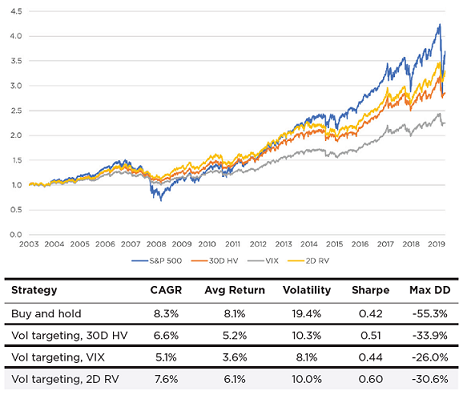
On this figure, the added value of high frequency data in terms of improved performances for the associated volatility targeting strategy is clear.

Daily volatility targeting for the SPY ETF using open/high/low/close intraday data

Figure 2 illustrates my reproduction of Figure 1, using two different volatility forecasting models:

• 30d HV - the volatility forecast³³ produced by the 30-day simple moving average of the square root of the daily squared close-to-close returns
• 2d JAPR - the volatility forecast³³ produced by the 2-day simple moving average of the daily jump-adjusted Parkinson range

Figure 2. Daily volatility targeting strategy for misc. volatility proxies, SPY ETF, December 2003 - March 2020.

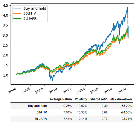
Comparing Figure 1 and Figure 2, it seems that performance metrics differ for buy and hold³⁴, so that an absolute comparison between the different volatility targeting strategies will not be possible.

Nevertheless, it is visible in Figure 2 that the volatility forecasting model based on the jump-adjusted Parkinson range exhibit a better volatility control and a slightly higher average return than the volatility forecasting model based on squared close-to-close returns.

While the relative improvement is not as dramatic as in Figure 1³⁵, this empirically demonstrates that using open/high/low/close intraday data can definitely be beneficial to a volatility targeting strategy.

Conclusion

In this blog post, I showed that simple volatility forecasting models can be useful in practice, especially when paired with range-based volatility estimators like the Parkinson estimator.

Next in this series dedicated to volatility forecasting, I will detail the reference model when it comes to volatility forecasting³⁶ - the GARCH model - and as usual, I will add my own twist to it.

Meanwhile, feel free to connect with me on LinkedIn or to follow me on Twitter.

–

1. The term returns is loosely defined here, but think for example daily close-to-close returns for daily volatility forecasting. ↩

2. See Andrew J. Patton, Volatility forecast comparison using imperfect volatility proxies, Journal of Econometrics, Volume 160, Issue 1, 2011, Pages 246-256. ↩ ↩² ↩³ ↩⁴

3. See Boudoukh, J., Richardson, M., & Whitelaw, R.F. (1997). Investigation of a class of volatility estimators, Journal of Derivatives, 4 Spring, 63-71. ↩ ↩² ↩³ ↩⁴ ↩⁵

4. See Figlewski, S. (1997), Forecasting Volatility. Financial Markets, Institutions & Instruments, 6: 1-88. ↩ ↩² ↩³ ↩⁴

5. Assuming the time period $t$ is of unit length. ↩

6. See Fischer Black, One Way to Estimate Volatility, Black on Options, Vol 1, No. 8, May 17, 1976. ↩

7. Indeed, it is extremely difficult to obtain an accurate mean estimate from the data⁴ and the real problem as far as volatility calculation is concerned is to avoid using extreme sample mean returns that will periodically be produced from short data samples⁴. ↩

8. In the statistical sense, c.f. Wikipedia. ↩

9. See Alizadeh, S., Brandt, M.W. and Diebold, F.X. (2002), Range-Based Estimation of Stochastic Volatility Models. The Journal of Finance, 57: 1047-1091. ↩

10. That being said, Brunetti and Lildholdt³⁷ showed that the conditions of validity of the Parkinson volatility estimator could be relaxed, allowing the process driving the asset returns to exhibit time-varying volatility and fat tails! ↩

11. See Richard D.F. Harris, Fatih Yilmaz, Estimation of the conditional variance-covariance matrix of returns using the intraday range, International Journal of Forecasting, Volume 26, Issue 1, 2010, Pages 180-194. ↩ ↩²

12. Which, by the way, is a stylized fact of volatility³⁸. ↩

13. By recursive substitution, an estimate of the asset next $h$-period’s ahead volatility $\hat{\sigma}_{T+h}$, $h \geq 2$, is a weighted moving average of that asset past periods variance proxies plus that asset past periods variance forecasts. ↩

14. See Lazard Asset Management, Predicting Volatility, December 2015. ↩ ↩² ↩³

15. See RiskMetrics. Technical Document, J.P.Morgan/Reuters, New York, 1996. Fourth Edition. ↩ ↩² ↩³ ↩⁴ ↩⁵ ↩⁶

16. See Fulvio Corsi, A Simple Approximate Long-Memory Model of Realized Volatility, Journal of Financial Econometrics, Volume 7, Issue 2, Spring 2009, Pages 174-196. ↩

17. See Brooks, Chris and Persand, Gitanjali (2003) Volatility forecasting for risk management. Journal of Forecasting, 22(1). pp. 1-22. ↩ ↩² ↩³ ↩⁴

18. There are other possible choices for the initial value $\hat{\sigma}_{0}^2. ↩

19. Other procedures are described in the RiskMetrics technical document¹⁵. ↩

20. See Axel A. Araneda, Asset volatility forecasting:The optimal decay parameter in the EWMA model, arXiv. ↩ ↩² ↩³ ↩⁴

21. These ETFs are used in the Adaptative Asset Allocation strategy from ReSolve Asset Management, described in the paper Adaptive Asset Allocation: A Primer³⁹. ↩

22. See Mincer, J. and V. Zarnowitz (1969). The evaluation of economic forecasts. In J. Mincer (Ed.), Economic Forecasts and Expectations. ↩

23. The common ending price history of all the ETFs is 31 August 2023, but there is no common starting price history, as all ETFs started trading on different dates. ↩

24. For the exponentially weighted moving average, I used an expanding window for the volatility forecast computation. ↩

25. In terms of lower $\alpha$, $\beta$ closer to 1 and higher $R^2$. ↩ ↩² ↩³ ↩⁴

26. Personally, I would recommend to use the exponentially weighted moving average model with the optimal decay factor $\lambda$ automatically determined. ↩

27. See Salt Financial, Risk Before Return: Targeting Volatility with Higher Frequency Data, Research Note. ↩ ↩² ↩³

28. Salt Financial people scale their proposed intraday high frequency realized volatility measure in order to account for overnight returns. ↩

29. See Andersen, T. G. and Bollerslev, T.: 1998, Answering the skeptics: Yes, standard volatility models do provide accurate forecasts, International Economic Review 39, 885-905. ↩

30. See Harvey, Campbell R. and Hoyle, Edward and Korgaonkar, Russell and Rattray, Sandy and Sargaison, Matthew and van Hemert, Otto, The Impact of Volatility Targeting. ↩ ↩²

31. Implemented with a one-day lag. ↩

32. That’s my understanding of the term “historical volatility” in the Salt Financial research note²⁷. ↩

33. At a 2-day horizon, due to the Salt Financial one-day lag implementation²⁷. ↩ ↩²

34. Probably because the research note from Salt Financial²⁷ uses excess returns whereas my reproduction uses raw returns. ↩

35. In Figure 1, the increase in terms of Sharpe ratio is 0.09, while in Figure 2, it is only 0.05. ↩

36. See Hansen, P.R. and Lunde, A. (2005), A forecast comparison of volatility models: does anything beat a GARCH(1,1)?. J. Appl. Econ., 20: 873-889. ↩

37. See Brunetti, Celso and Lildholdt, Peter M., Return-Based and Range-Based (Co)Variance Estimation - with an Application to Foreign Exchange Markets (March 2002). ↩

38. See R. Cont (2001) Empirical properties of asset returns: stylized facts and statistical issues, Quantitative Finance, 1:2, 223-236. ↩

39. See Butler, Adam and Philbrick, Mike and Gordillo, Rodrigo and Varadi, David, Adaptive Asset Allocation: A Primer. ↩