Mean-Variance Optimization in Practice: Subset Resampling-based Efficient Portfolios

10 minute read

In a previous post, I introduced near efficient portfolios, which are portfolios equivalent to mean-variance efficient portfolios in terms of risk-return but more diversified in terms of asset weights.

Such near efficient portfolios might be used to moderate the tendency of efficient portfolios to be concentrated in a very few assets, a well-known stylized fact of the Markowitz’s mean-variance framework¹.

Another stylized fact of the Markowitz’s mean-variance framework is the sensitivity of efficient portfolios to estimation error in asset returns and (co)variances², which explains why efficient portfolios are sometimes labeled estimation-error maximizers³.

In this new post, I will explore a solution to this problem based on a machine learning technique called the random subspace method, initially introduced by David Varadi from CSS Analytics under the name random subspace optimization (RSO)⁴ and later re-discovered independently by Benjamin J. Gillen under the name subset optimization⁵ and by Weiwei Shen and Jun Wan under the name subset resampling⁶⁷.

Notes:

A Google Sheet corresponding to this post is available here

Update (May 2023): The machine learning technique described in this post is publicly used in the financial industry, c.f. Parala SOL Indices

Mathematical preliminaries

Definition

The random subspace method is an ensemble learning technique, introduced in Ho⁸ in the context of decision trees, that combines the predictions from multiple machine learning models trained independently on different random subspaces of the feature space.

More formally, it consists in the following steps:

Determine the common size $n_S$ of the random subspaces, with $2 \le n_S \le n-1$ where $n$ is the size of the feature space
Determine the number of random subspaces $n_B$ to generate, with $1 \le n_B$
For $b = 1..n_B$ do
- Generate uniformly at random without replacement a $n_S$-dimensional subspace from the original $n$-dimensional feature space
- Compute a machine learning model $M_b$ using the whole training dataset projected onto the generated $n_S$-dimensional subspace⁹
Combine the $n_B$ machine learning models $M_1,..,M_{n_B}$ by averaging, the averaging procedure depending on the exact machine learning models (regression, classification, etc.)

Rationale

When the size of a training dataset is small compared to the dimensionality of the feature space, it is difficult to train a machine learning model because there is not enough data to accurately estimate the model parameters.

This problem, sometimes referred as the curse of dimensionality, usually results in¹⁰:

The model being biased with high variance
The model being unstable, with small changes in the input data causing large changes in the model predictions

The random subspace method is a possible solution to this problem thanks to the relative increase in the size of the training dataset that it creates¹¹.

From this perspective, the random subspace method is a dimensionality reduction method designed to combat the curse of dimensionality⁸.

Computing subset resampling-based mean-variance efficient portfolios

Random subspace method meets mean-variance optimization

For a universe of $n$ assets, mean-variance optimization requires the estimates of the following parameters:

$n$ asset returns
$n$ asset variances
$\frac{n (n-1)}{2}$ asset correlations

In other words, the dimension of the feature space associated to mean-variance optimization grows quadratically with the number of assets.

This implies, because the historical data typically used for estimating the above parameters grows only linearly with the number of assets¹², that mean-variance optimization is subject to the curse of dimensionality.

In addition, there is usually some redundancy in any universe of assets due to highly correlated assets (e.g. U.S. equities and World equities, Bitcoin and Ethereum cryptocurrencies…), which is an independent source of instability in mean-variance optimization named instability caused by signal in Lopez de Prado¹³.

The random subspace method is able to address these two problems:

It is designed to combat the curse of dimensionality, as mentioned in the previous section
It is known to produce robust models when features are redundant⁸

So, the random subspace method seems to be a promising approach in the context of mean-variance optimization!

Algorithm overview

Formally, when applied to mean-variance optimization in a universe of $n$ assets, the random subspace method consists in the following steps:

Determine the number of assets $n_S$ to include in each random subset of assets, with $2 \le n_S \le n-1$
Determine the number of random subsets of assets $n_B$ to generate, with $1 \le n_B$
For $b = 1..n_B$ do
- Generate uniformly at random without replacement a subset of $n_S$ assets from the original set of $n$ assets
- Compute the weights $w_b^{*}$ of a mean-variance efficient portfolio associated to the generated subset of $n_S$ assets, taking into account applicable constraints (return/volatility constraint, weight constraints…)
Combine the $n_B$ portfolio weights $ w_{1}^{*},..,w_{n_B}^{*} $ by averaging them through the formula $w^{*} = \frac{1}{n_B} \sum_{b=1}^{n_B} w_b^{*}$

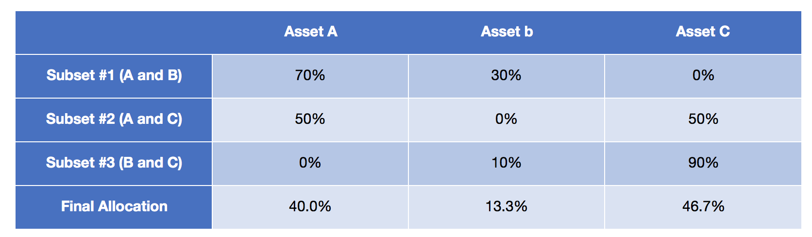
Figure 1, taken from the Flirting with Models blog post Machine Learning, Subset Resampling, and Portfolio Optimization illustrates these steps in a 3-asset universe with the enumeration of all the 2-asset subsets.

Figure 1. Random subspace method applied to mean-variance optimization. Source: Flirting with Models

Portfolio Optimizer implementation

Portfolio Optimizer provides 4 endpoints to compute subset resampling-based mean-variance efficient portfolios:

They all share some common important implementation details, that are described below.

Step 1: Determination of the number of assets to include in each random subset of assets

Gillen⁵ and Shen and Wan⁶ note that there is a trade-off between diversification benefits and estimation risk when varying $n_S$.

As Shen and Wan put it⁶:

The smaller the subset size is, the more accurate the estimation of the sample covariance matrix would be, yet the more diversification benefits would be lost, and vice versa.

While nothing can be said in general about how to best achieve this trade-off¹⁴, Shen and Wan⁶ empirically show that a value of $n_S\in [0.6, 0.8]$ allows to achieve good performances on several universes of assets.

Portfolio Optimizer uses by default a proprietary value for $n_S$ whose order of magnitude is $\sqrt{n}$, similar in spirit to the square root rule used when creating a random forest¹⁵.

Step 2: Determination of the number of random subsets of assets to generate

Gillen⁵ addresses the issue of determining a proper value for $n_B$:

Theoretically, using the law of large numbers, he notes that a reasonably large value for $n_B$ allows the combined portfolio weights $w^{*}$ to converge
Practically, he suggests that

the number of subsets could be determined so that each security appears in a fixed number of subset portfolios. For instance, if each security is selected into 10,000 subset portfolios, then the standard error of its weight due to subset selection will reduced by a factor of 1%. Such a specification would suggest generating $10000 \frac{n}{n_S}$ subsets

Portfolio Optimizer uses by default a value of 128 for $n_B$, based on a paper from Oshiro et al. on random forests¹⁶.

Notes:

The total number of subsets containing $n_S$ assets in a universe of $n$ assets is equal to $\frac{n!}{n_S!(n - n_S)!}$. Combinatorial explosion makes it impossible to compute all these subsets, so that generating a fixed number $n_B$ of them is usually required in practice.

Nevertheless, when the value of $\frac{n!}{n_S!(n - n_S)!}$ is relatively small, for example when $n \approx 15$, Portfolio Optimizer is able to compute all these subsets if required, in which case determining $n_B$ is not necessary.

Step 3: Computation of a mean-variance efficient portfolio associated to a random subset of assets

This step is straightforward, except for the management of constraints.

Indeed, while Gillen⁵ states that

incorporating constraints into the optimization problem is mainly a computational issue

, it is actually possible that the constraints imposed on a universe of $n$ assets are such that the mean-variance optimization problem associated to any subset of $n_S < n$ assets is infeasible¹⁷.

In order to ensure that enough feasible random subsets are generated, Portfolio Optimizer allows a maximum proportion of 5% of infeasible random subsets over the total number of generated random subsets.

Step 4: Combination of the subset mean-variance efficient portfolios

Gillen⁵ shows that combining the subset mean-variance efficient portfolios by averaging their weights is an ex-ante optimal weighting scheme.

That being said, there are other possible weighting schemes, like for example combining the subset mean-variance efficient portfolios through the usage of a robust measure of location called the geometric median.

The geometric median might be an interesting weighting scheme because it is less sensitive than the arithmetic mean to unstable selection of assets and it has been empirically demonstrated to be effective in machine learning applications under the name of bragging¹⁸.

Portfolio Optimizer allows to use these two weighting schemes, the default one being the averaging weighting scheme.

Performance analysis of subset resampling-based mean-variance efficient portfolios

Raw and risk-adjusted performances of the random subspace method applied to mean-variance optimization have been analyzed:

In the CSS Analytics blog post RSO MVO vs Standard MVO Backtest Comparison
In Gillen⁵
In Shen and Wan⁶
In the Flirting with Models blog post Machine Learning, Subset Resampling, and Portfolio Optimization

In a large majority of backtests, subset resampling-based mean-variance efficient portfolios have been found to outperform equal-weighted portfolios and mean-variance efficient portfolios.

I initially wanted to reproduce one of these backtests in this post, but I finally decided to highlight another aspect of these portfolios.

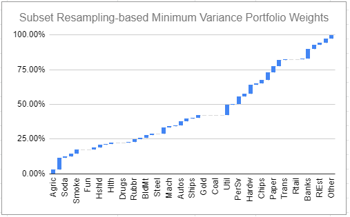
Figures 2 and 3 illustrate the typical asset weights of a minimum variance portfolio v.s. a subset resampling-based minimum variance portfolio, both computed using the $n = 49$ industry portfolios provided in the Fama and French data library¹⁹.

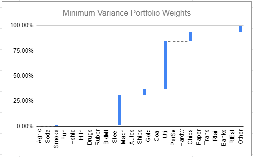
Figure 2. Minimum variance portfolio weights.

Figure 3. Subset resampling-based minimum variance portfolio weights.

As expected, the minimum variance portfolio is heavily concentrated in a few industries - about 6.

Maybe less expected, though, is that the subset resampling-based minimum variance portfolio is extremely well diversified in terms of industries despite no maximum weight constraints imposed.

So, not only subset resampling-based mean-variance efficient portfolios are able to outperform both equal-weighted portfolios and mean-variance efficient portfolios²⁰, but such portfolios are also far more diversified in terms of asset weights than their vanilla counterparts!

Limitations of subset resampling-based mean-variance efficient portfolios

There are two main issues with the random subspace method applied to mean-variance optimization as presented in this post:

The subsets of assets are generated at random, so that the computed portfolios weights change every time a new optimization is performed.

Generating a high number of subsets $n_B$ and combining the subset mean-variance efficient portfolios thanks to the geometric median are two possible and complementary ways to alleviate this issue.

Unfortunately, nothing else can be done, because as Gillen puts it⁵, sacrificing some benefits of the textbook mean-variance optimization is required in order to mitigate the risk of estimation error.

The subsets of assets are generated uniformly at random, so that the method is sensitive to the universe of assets

An illustrative example for this one.

If a universe of 10 assets contains:

6 equity-like assets
3 bond-like assets
1 commodity-like asset

Then:

The probability that an equity-like asset is selected as part of any subspace of assets is $6/10 = 60$%
The probability that a bond-like asset is selected as part of any subspace of assets is $3/10 = 30$%
The probability that a commodity-like asset is selected as part of any subspace of assets is $1/10 = 10$%

So, the combined portfolio will be over-concentrated in equity-like assets.

More generally, if a universe of assets contains a large number of assets belonging to the same asset class, the combined portfolio will be over-concentrated in this asset class.

This issue, together with an elegant solution, was described initially in the CSS Analytics blog post Cluster Random Subspace Method for Portfolio Management, and will be the subject of another post.

Meanwhile, happy resampling !

–

See F. Black and R. Litterman, Global Portfolio Optimization, Financial Analysts Journal, Vol. 48, No. 5 (Sep. - Oct., 1992), pp. 28-43. ↩
See Broadie, M. Computing efficient frontiers using estimated parameters. Ann Oper Res 45, 21–58 (1993). ↩
See Michaud, Richard O., The Markowitz Optimization Enigma: Is ‘Optimized’ Optimal? (1989). Financial Analysts Journal, 1989. ↩
See Random Subspace Optimization (RSO). ↩
See Gillen, Benjamin J. (2016) Subset Optimization for Asset Allocation. Social Science Working Paper, 1421. California Institute of Technology , Pasadena, CA. ↩ ↩² ↩³ ↩⁴ ↩⁵ ↩⁶ ↩⁷
See Shen, Weiwei and Wang, Jun, Portfolio selection via subset resampling, AAAI’17: Proceedings of the Thirty-First AAAI Conference on Artificial Intelligence, Pages 1517–1523. ↩ ↩² ↩³ ↩⁴ ↩⁵
Portfolio Optimizer uses the term subset resampling. ↩
See Tin Kam Ho, “The random subspace method for constructing decision forests,” in IEEE Transactions on Pattern Analysis and Machine Intelligence, vol. 20, no. 8, pp. 832-844, Aug. 1998. ↩ ↩² ↩³
As an example, this projection usually forces numerical features in the unselected dimensions to 0. ↩
See Skurichina, M., Duin, R. Bagging, Boosting and the Random Subspace Method for Linear Classifiers. Pattern Anal Appl 5, 121–135 (2002). ↩
The size of the training dataset is relatively increased because the dimension of the random subsets is smaller than the dimension of the original feature space while the size of the training dataset is kept constant. ↩
With $T$ the common length of historical data across all the assets (e.g. $T = 252$ days, etc.), the total size of historical data grows linearly with the number of assets as $n T$. ↩
See Lopez de Prado, Marcos, A Robust Estimator of the Efficient Frontier (October 15, 2016). ↩
Although both Gillen⁵ and Shen and Wan⁶ note that it is preferable that $n_S < min(n, T)$, with $T$ the common length of historical data across all the assets used to estimate the asset covariance matrix. ↩
See sklearn.ensemble.RandomForestClassifier. ↩
See Oshiro, T.M., Perez, P.S., Baranauskas, J.A. (2012). How Many Trees in a Random Forest?. In: Perner, P. (eds) Machine Learning and Data Mining in Pattern Recognition. MLDM 2012. Lecture Notes in Computer Science(), vol 7376. Springer, Berlin, Heidelberg. ↩
This is typically the case for weight constraints, but the same remark applies to the return/volatility constraint associated to the mean-variance optimization problem. ↩
bragging stands for bootstrap robust aggregation, c.f. Buhlmann²¹. ↩
I chose $n_S$ to be the default value computed by Portfolio Optimizer, $n_B = 16384$ and a 12-month window to compute the covariance matrix of the monthly returns of the 49 industries. ↩
This outperformance is not found to be statistically significant in terms of Sharpe ratio in the Flirting with Models blog post, but it definitely is in Shen and Wan⁶. ↩
See Peter Buhlmann, Bagging, Subagging and Bragging for Improving some Prediction Algorithms, Recent Advances and Trends in Nonparametric Statistics, JAI, 2003, Pages 19-34. ↩