Covariance Matrix Forecasting: Average Oracle Method

Continuing this series on covariance matrix forecasting (c.f. here and there for the previous posts), I will now describe a relatively recent¹ data-driven, model-free, way to [forecast] covariance [and correlation] matrices of time-varying systems² rooted in random matrix theory.

This method - introduced in Bongiorno et al.² and called Average Oracle - consists in replacing the eigenvalues of a (noisy) estimate of a time-varying covariance matrix by time-independant eigenvalues that encode the average influence of the future on present eigenvalues².

In this blog post, I will describe that method and, as now usual in this series, I will illustrate its empirical performances in the context of monthly covariance matrix forecasting for a multi-asset class ETF portfolio.

Mathematical preliminaries

Some of these sub-sections contain reminders from a previous blog post.

Dynamic covariance and correlation matrices

Let $n$ be the number of assets in a universe of assets and $r_t \in \mathbb{R}^n$ be the vector of the (logarithmic) return process of these assets over a time period $t$ (a day, a week, a month..) over which their mean return vector $\mu_t \in \mathbb{R}^n$ is supposed to be null.

Then:

• The asset covariance matrix $\Sigma_t \in \mathcal{M}(\mathbb{R}^{n \times n})$ over the time period $t$ is defined as $\Sigma_t = \mathbb{E} \left[ r_t r_t {}^t \right]$.

  That matrix is called³ the population (or true) covariance matrix of the asset returns over the time period $t$.

• The asset correlation matrix $C_t \in \mathcal{M}(\mathbb{R}^{n \times n})$ over the time period $t$ is defined as the correlation matrix $ C_t = V_t^{-1} \Sigma_t V_t^{-1} $ associated to the covariance matrix $\Sigma_t$, where $V_t \in \mathcal{M}(\mathbb{R}^{n \times n})$ is the diagonal matrix of the asset standard deviations.

Let now be $T$ time periods $t = 1..T$.

Then:

• The averaged⁴ covariance matrix $\Sigma_{1:T} \in \mathcal{M}(\mathbb{R}^{n \times n})$ over the $T$ time periods $t = 1..T$ is defined as $ \Sigma_{1:T} = \frac{1}{T} \sum_{t=1}^{T} \Sigma_{t} $.

  In case the return process is time-invariant, the averaged covariance matrix $\Sigma_{1:T}$ is equal to the (constant) population covariance matrix $\left( \Sigma = \right) \Sigma_t, t = 1..T$.

• The averaged⁴ correlation matrix $C_{1:T} \in \mathcal{M}(\mathbb{R}^{n \times n})$ over the $T$ time periods $t = 1..T$ is defined as $ C_{1:T} = \frac{1}{T} \sum_{t=1}^{T} C_{t} $.

  In case the return process is time-invariant, the averaged correlation matrix $C_{1:T}$ is equal to the (constant) correlation matrix $\left( C = \right) = C_t, t = 1..T$.

• The pseudo-averaged⁵ correlation matrix $C_{p, 1:T} \in \mathcal{M}(\mathbb{R}^{n \times n})$ over the $T$ time periods $t = 1..T$ is defined as the correlation matrix associated to the averaged covariance matrix $\Sigma_{1:T}$.

  In case the return process is time-invariant, the pseudo-averaged correlation matrix $C_{p, 1:T} $ is equal to the averaged correlation matrix $C_{1:T}$, but in general, due to time-varying asset standard deviations, the two correlation matrices are different.

Dynamic covariance and correlation matrices sample estimators

In practice, the asset return process $r_t$ is usually not known and the only available information is the vectors of realized asset returns $ \tilde{r}_1,…, \tilde{r}_T \in \mathbb{R}^n$ for $T$ time periods.

From each of these vectors:

• The classical way to estimate the covariances is to compute the empirical (or sample) covariance matrix thanks to Pearson estimator³ defined as $\tilde{\Sigma}_t = \tilde{r}_t \tilde{r}_t {}^t $ over each time period $t = 1..T$.

  Here, the outer product of the realized asset returns $ \tilde{r}_t \tilde{r}_t {}^t $ over the time period $t$ is called a covariance estimate $\tilde{\Sigma}_t$ - or covariance proxy⁶ - for the (unobserved) asset returns covariance matrix over that time period.

• The empirical (or sample) correlation matrix over each time period $t = 1..T$ is defined as the correlation matrix $ \tilde{C}_t $ associated to the covariance matrix $\tilde{\Sigma}_t$.

• The empirical averaged covariance matrix over the $T$ time periods $t = 1..T$ is typically estimated from the realized asset returns $ \tilde{r}_1,…, \tilde{r}_T \in \mathbb{R}^n$ thanks to the averaged Pearson estimator defined as $\tilde{\Sigma}_{1:T} = \frac{1}{T} \sum_{t=1}^{T} \tilde{r}_t \tilde{r}_t {}^t $.

• The empirical averaged correlation matrix over the $T$ time periods $t = 1..T$ is defined as $ \tilde{C}_{1:T} = \frac{1}{T} \sum_{t=1}^{T} \tilde{C}_{t} $.

• The empirical pseudo-averaged correlation matrix over the $T$ time periods $t = 1..T$ is defined as the correlation matrix $ \tilde{C}_{p, 1:T}$ associated to the empirical averaged covariance matrix $\tilde{\Sigma}_{1:T}$.

Covariance and correlation matrices rotationally invariant estimators

Rotationally invariant estimators

As already mentioned in a previous blog post on correlation matrices denoising, the estimation of empirical covariance and correlation matrices in finance is affected by noise, in the form of measurement error, due in part to the short length of the time series of asset returns typically used in their computation.

Indeed:

• Constructing a well-diversified portfolio requires many assets⁷, that is, a big $n$.
• In contrast, rapid shifts in financial market dependencies can only be captured by short calibration windows⁷ for estimating asset correlations, that is, a small $T$.

This situation leads to an aspect ratio $q = \frac{n}{T}$ of empirical matrices either close to 1 - or even worse, much greater than 1 -, which is catastrophic from an estimation perspective, c.f. the above blog post and references therein.

Hopefully, numerous techniques have been developed to improve the estimation of noisy covariance [or correlation] matrices⁷.

Several of these techniques, like the eigenvalue clipping method⁸, involve a specific class of matrix estimators - known as Rotationally Invariant Estimators (RIE) or Orthogonally Invariant Estimators (OIE) - that leaves the eigenvectors of the empirical matrices untouched while altering their eigenvalues.

In other words, an RIE estimator $\Xi \left( \tilde{\Sigma}_t \right) \in \mathcal{M}(\mathbb{R}^{n \times n})$ of a true covariance or correlation matrix $\Sigma_t \in \mathcal{M}(\mathbb{R}^{n \times n})$ obtained from its empirical counterpart $\tilde{\Sigma}_t \in \mathcal{M}(\mathbb{R}^{n \times n})$ has the general form

\[\Xi \left( \tilde{\Sigma}_t \right) = \tilde{V}_t \Lambda_t \tilde{V}_t {}^t\]

, where:

• $\Lambda_t \in \mathcal{M}(\mathbb{R}^{n \times n})$ is a diagonal matrix of well-chosen² eigenvalues.
• $\tilde{V}_t \in \mathcal{M}(\mathbb{R}^{n \times n})$ is the matrix of eigenvectors of $\tilde{\Sigma}_t$, defined through the spectral decomposition $ \tilde{\Sigma}_t = \tilde{V}_t \tilde{\Lambda}_t \tilde{V}_t {}^t $ with $ \tilde{\Lambda}_t \in \mathcal{M}(\mathbb{R}^{n \times n})$ the diagonal matrix of eigenvalues of $\tilde{\Sigma}_t$.

Bun et al.³ explains the underlying rationale as follows:

The true matrix [$\Sigma_t$] is unknown and we do not have any particular insights on its components (the eigenvectors).

Therefore we would like our estimator [$\Xi \left( \tilde{\Sigma}_t \right)$] to be constructed in a rotationally invariant way from the noisy observation [$\tilde{\Sigma}_t$] that we have.

In simple terms, this means that there is no privileged direction in the $n$-dimensional space that would allow one to bias the eigenvectors of the estimator [$\Xi \left( \tilde{\Sigma}_t \right)$] in some special directions.

More formally, the estimator construction must obey: $ \Omega \Xi \left( \tilde{\Sigma}_t \right) \Omega {}^t$ $=$ $\Xi \left( \Omega \tilde{\Sigma}_t \Omega {}^t \right)$ for any rotation matrix $\Omega \in \mathcal{M}(\mathbb{R}^{n \times n})$.

Any estimator satisfying [that equation] will be referred to as a Rotational Invariant Estimator (RIE).

In this case, it turns out that the eigenvectors of the estimator [$\Xi \left( \tilde{\Sigma}_t \right)$] have to be the same as those of the noisy matrix [$\tilde{\Sigma}_t$].

Rotationally invariant oracle estimator

Bun et al.³ shows that the optimal RIE estimator of the unknown matrix $\Sigma_t$ in terms of Frobenius norm is the RIE estimator whose diagonal matrix of eigenvalues $\Lambda_O$ satisfy

\[\Lambda_O = \text{diag} \left( \tilde{V}_t {}^t \Sigma_t \tilde{V}_t \right)\]

That estimator is sometimes called the oracle estimator because it depends explicitly on the knowledge of the true signal [$\Sigma_t$]³ and so is not directly usable in practice.

Remarkably, [though], asymptotically optimal RIEs that converge to the oracle estimator can be obtained without the knowledge of the true covariance; however, such estimators require that: i) the ground truth does not change, ii) the data matrix is very large, and iii) the data has at least finite fourth moments².

Those conditions, and especially the first one, are definitely not satisfied by asset returns, which leads to suboptimal estimators in practice…

As a side note, and maybe contrary to intuition, the optimal eigenvalues $\Lambda_O$ are NOT equal to the eigenvalues of $\Sigma_t$, because this would result in a spectrum that is too wide³.

The Average Oracle covariance matrix forecasting method

Forecasting formulas

Let be:

• $n$ be the number of assets in a universe of assets
• $\tilde{r}_t \tilde{r}_t {}^t$, $t=1..T$ the outer products of the observed asset returns over each of $T$ past periods
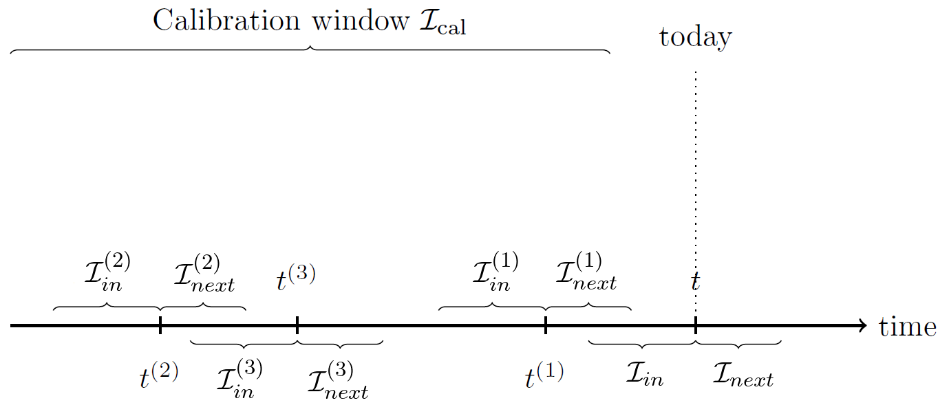
• $1 \leq h_{in} \ll T$ a chosen number of past periods
• $\mathcal{I}_{cal} = [t_{cal}, T - h_{next}]$ a long calibration window, with $t_{cal}$ chosen so that $t_{cal} \geq h_{in} - 1$ and $| \mathcal{I}_{cal} | \gg h_{in}$

Asset returns averaged covariance matrix

The Average Oracle covariance matrix forecasting model estimates the asset returns averaged covariance matrix $\hat{\Sigma}_{T+1:T+h_{next}}$ over the next $h_{next} \geq 1$ periods as follows²:

• Choose a number of random time periods $n_B \geq 1$ to generate.

• For $b = 1..n_B$ do

  • Select uniformly at random with replacement a time period $t^{(b)} \in \mathcal{I}_{cal}$

  • Compute the “past” averaged asset returns covariance matrix $ \tilde{\Sigma}^{(b)}_{in} $ on the train window $\mathcal{I}^{(b)}_{in} = [t^{(b)} - h_{in} + 1, t^{(b)}]$, defined by $\tilde{\Sigma}^{(b)}_{in} = \tilde{\Sigma}_{t^{(b)} - h_{in} + 1:t^{(b)}} = \frac{1}{h_{in}} \sum_{t=t^{(b)} - h_{in} + 1}^{t^{(b)}} \tilde{r}_t \tilde{r}_t {}^t $ and its associated correlation matrix $\tilde{C}^{(b)}_{in} = \tilde{C}_{p, t^{(b)} - h_{in} + 1:t^{(b)}}$ whose spectral decomposition is given by $\tilde{C}^{(b)}_{in} = \tilde{V}^{(b)}_{in} \tilde{\Lambda}^{(b)}_{in} \tilde{V}^{(b)}_{in} {}^t $.

  • Compute the “future” averaged asset returns covariance matrix $ \tilde{\Sigma}^{(b)}_{next} $ on the test window $\mathcal{I}^{(b)}_{next} = [t^{(b)} + 1, t^{(b)} + h_{next}]$, defined by $ \tilde{\Sigma}^{(b)}_{next} = \tilde{\Sigma}_{t^{(b)} + 1:t^{(b)} + h_{next}} = \frac{1}{h_{next}} \sum_{t=t^{(b)} + 1}^{t^{(b)} + h_{next}} \tilde{r}_t \tilde{r}_t {}^t $ and its associated correlation matrix $\tilde{C}^{(b)}_{next} = \tilde{C}_{p, t^{(b)} + 1:t^{(b)} + h_{next}}$.

  • Compute the diagonal matrix of oracle eigenvalues $\tilde{\Lambda}_O^{(b)} = \text{diag} \left( \tilde{V}^{(b)}_{in} {}^t \tilde{C}^{(b)}_{next} \tilde{V}^{(b)}_{in} \right) $.

• Compute the diagonal matrix of Average Oracle eigenvalues $\tilde{\Lambda}_{AO} = \frac{1}{n_B} \sum_{b=1}^{n_B} \tilde{\Lambda}_O^{(b)} $.

• Compute the most recent “past” averaged asset returns covariance matrix $ \tilde{\Sigma}_{in} $ on the window $\mathcal{I}_{in} = [T - h_{in} + 1, T]$, defined by $ \tilde{\Sigma}_{in} = \tilde{\Sigma}_{T - h_{in} + 1:T} = \frac{1}{h_{in}} \sum_{t=T - h_{in} + 1}^{T} \tilde{r}_t \tilde{r}_t {}^t $ and its associated correlation matrix $\tilde{C}_{in} = \tilde{C}_{p, T - h_{in} + 1:T}$ whose spectral decomposition is given by $\tilde{C}_{in} = \tilde{V}_{in} \tilde{\Lambda}_{in} \tilde{V}_{in} {}^t $.

• Compute $\hat{\Sigma}_{T+1:T+h_{next}} = D_{in} \tilde{V}_{in} \tilde{\Lambda}_{AO} \tilde{V}_{in} {}^t D_{in} $, where $D_{in} \in \mathcal{M}(\mathbb{R}^{n \times n})$ is the diagonal matrix of the standard deviations $\sqrt{ \left( \tilde{\Sigma}_{in} \right)_ii }, i=1..n$.

For more visual clarity, Figure 1 illustrates that process.

Figure 1. Illustration of the Average Oracle eigenvalues computation process, which uses different windows included in a long calibration window. Source: Adapted from Bongiorno et al.

Asset returns averaged and pseudo-averaged correlation matrix

The Average Oracle covariance matrix forecasting model does not easily⁹ allow to estimate the asset returns averaged correlation matrix $\hat{C}_{T+1:T+h_{next}}$, because it does not rely on the estimation of the individual covariance matrices $\hat{\Sigma}_{T+1}$, $…$, $\hat{\Sigma}_{T+h_{next}}$.

The asset returns pseudo-averaged correlation matrix $\hat{C}_{p, T+1:T+h_{next}}$ over the next $h_{next}$ periods, though, corresponds to the correlation matrix associated to the averaged covariance matrix $\hat{\Sigma}_{T+1:T+h_{next}}$.

Rationale

The Average Oracle covariance matrix forecasting method captures the average transition from two consecutive time windows² by averaging [oracle eigenvalues], rank-wise, over many randomly selected consecutive intervals taken from a long calibration window².

That covariance matrix forecasting method thus tackles the evolution of [asset returns] dependencies with a time-invariant eigenvalue cleaning scheme².

As noted in Bongiorno et al.²:

This is a zeroth order approximation, as the fluctuations of the optimal eigenvalue matrix around $\tilde{\Lambda}_{AO}$ sometimes most probably contain valuable additional information (as may do those of the eigenvectors). Nevertheless, this approximation is a powerful filtering tool and is easily computed from data without any modeling assumptions about the underlying system.

Performances

From a practical perspective, Bongiorno et al.² and Bongiorno and Challet¹⁰ empirically demonstrate that the Average Oracle covariance matrix forecasting method is more performant than the current state-of-the-art (and complex) methods, Dynamic Conditional Covariance coupled to Non-Linear Shrinkage (DCC+NLS)¹⁰, both in terms of Frobenius distance - as highlighted in Figure 2 - and in terms of four key portfolio metrics: Sharpe ratio, turnover, gross leverage, and diversification¹⁰.

Figure 2. Average Frobenius distance between the forecasted and the out-of-sample covariance matrices of n = 100 U.S. stocks as a function of the number of past periods $h_{in}$. Source: Adapted from Bongiorno et al.

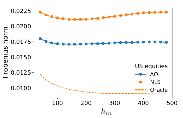
These performances are commented as follows in Bongiorno et al.²:

The fact that the Average Oracle is a better estimator for time-evolving covariance matrices most often implies that the most recent information contained in the sample eigenvalues is less relevant (and more noisy) than the AO ones that focus on the average transition.

Thus, the advantage of the Average Oracle is precisely that it captures some part of the average dynamics that is discarded by the assumption of a constant true covariance matrix [made in the DCC+NLS method].

Implementation details

How to choose the number of past periods $h_{in}$?

Through extensive simulations, Bongiorno et al.² concludes that the Average Oracle eigenvalues $\tilde{\Lambda}_{AO}$ mainly depend on the number of assets $n$ and¹¹ on the number of past periods $h_{in}$ over which to compute the averaged asset returns covariance matrix.

A natural question - unfortunately neither answered in Bongiorno et al.² nor in Bongiorno and Challet¹⁰ - is then how to choose the value of $h_{in}$ in order to obtain the best forecasting performances?

One possible answer, that relies on the interpretation of the Average Oracle covariance matrix forecasting method as a covariance matrix cleaning scheme², is to select $h_{in}$ so as to maximize the forecasting performances of a simple moving average covariance matrix forecasting model with a window size equal to $h_{in}$ for the considered value of $h_{next}$.

How to choose the number of random time periods $n_B$?

The number of random time periods $n_B$ must be high enough to ensure that the Average Oracle eigenvalues are stable enough - in particular when $h_{next}$ is small - because by reducing [$h_{next}$], the estimation becomes noisier and thus requires more train and test windows […] to yield average eigenvalues with the same level of precision².

Two examples¹²:

• Bongiorno et al.² uses $n_B = 10 000$ together with $h_{in} = h_{next} = 252$.
• Bongiorno and Challet¹⁰ uses $n_B = 10 000$ together with $h_{in} \in \lbrace 240, 1200 \rbrace$ and $h_{next} \in \lbrace 5, 20 \rbrace$.

To be noted, though, that depending on the length of the calibration window $\mathcal{I}_{cal}$ and/or on the number of assets $n$, the time periods do not need to be generated at random - they can perfectly be generated deterministically so as to cover the whole calibration window.

How to enforce a proper ordering of the Average Oracle eigenvalues?

Bongiorno et al.² stresses that the columns of the eigenvectors [$\tilde{V}^{(b)}_{in}$ and $\tilde{V}_{in}$] must always follow the same the eigenvalue ordering convention².

Nevertheless, despite enforcing such a convention, the order of the resulting Average Oracle eigenvalues $\tilde{\Lambda}_{AO}$ is not necessarily preserved due to the finite size of the sample¹³.

This may be an unwanted feature within a rotational invariant assumption¹³, since there is no reason a priori to expect that it is optimal to modify the order of the eigenvalues, that is to say, the variance associated with the principal components¹³.

Bun et al.¹³ proposes two solutions to this problem:

• Sort the resulting eigenvalues

• Perform an isotonic regression on the resulting eigenvalues

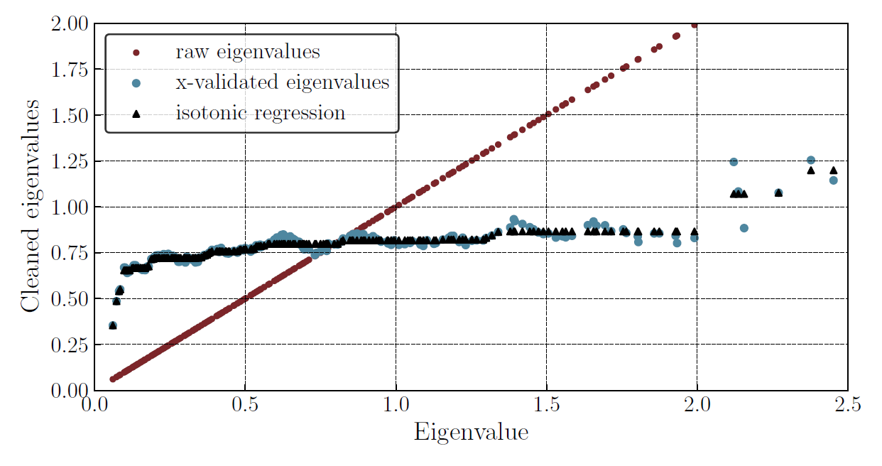
  In the context the cross-validated eigenvalues cleaning scheme described in Reigneron et al.¹⁴, the impact of using an isotonic regression is depicted in Figure 3.

  

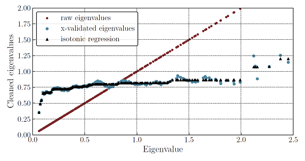
  Figure 3. Raw, cross-validated and isotonic eigenvalues eigenvalues as a function of in-sample eigenvalues. Source: Reigneron et al.

Implementation in Portfolio Optimizer

Portfolio Optimizer implements the Average Oracle covariance and correlation matrix forecasting models through the endpoints /assets/covariance/matrix/forecast/average-oracle and /assets/correlation/matrix/forecast/average-oracle.

These endpoints support the 2 covariance proxies below:

• Squared (close-to-close) returns
• Demeaned squared (close-to-close) returns

These endpoints also:

• Implement an isotonic regression correction step for the Average Oracle eigenvalues.
• Allow to automatically determine the number of past periods $h_{in}$, using a proprietary procedure.
• Allow to either generate a given number of time periods $n_B$ uniformly at random within the calibration window $\mathcal{I}_{cal}$ or use all the time periods available within that window.

Example of usage - Covariance matrix forecasting at monthly level for a portfolio of various ETFs

As an example of usage, I propose to evaluate the empirical performances of the Average Oracle covariance matrix forecating model within the framework of the previous blog bost, whose aim is to forecast monthly covariance and correlation matrices for a portfolio of 10 ETFs representative¹⁵ of misc. asset classes:

• U.S. stocks (SPY ETF)
• European stocks (EZU ETF)
• Japanese stocks (EWJ ETF)
• Emerging markets stocks (EEM ETF)
• U.S. REITs (VNQ ETF)
• International REITs (RWX ETF)
• U.S. 7-10 year Treasuries (IEF ETF)
• U.S. 20+ year Treasuries (TLT ETF)
• Commodities (DBC ETF)
• Gold (GLD ETF)

Results - Covariance matrix forecasting

Results over the period 31st January 2008 - 31st July 2023¹⁶ for covariance matrices are the following¹⁷:

Covariance matrix model	Covariance matrix MSE
SMA, window size of all the previous months (historical average model)	9.59 $10^{-6}$
SMA, window size of the previous year	9.08 $10^{-6}$
Average Oracle, optimal18 $h_{in}$	6.77 $10^{-6}$
EWMA, optimal18 $\lambda$	6.52 $10^{-6}$
IEWMA, optimal18 $\left(\lambda_{vol},\lambda_{cor}\right)$	6.16 $10^{-6}$
SMA, window size of the previous month (random walk model)	6.06 $10^{-6}$

Within this specific evaluation framework, the Average Oracle covariance matrix forecasting model¹⁹ unfortunately does not seem to exhibit improved performances v.s. much simplier models, like the EWMA covariance matrix forecasting model.

Results - Correlation matrix forecasting

Results over the period 31st January 2008 - 31st July 2023¹⁶ for the correlation matrices associated to the covariance matrices of the previous sub-section are the following¹⁷:

Covariance matrix model	Correlation matrix MSE
SMA, window size of the previous month (random walk model)	8.19
SMA, window size of all the previous months (historical average model)	8.10
Average Oracle, optimal18 $h_{in}$	6.59
SMA, window size of the previous year	6.50
EWMA, optimal18 $\lambda$	5.87
IEWMA, optimal18 $\left(\lambda_{vol},\lambda_{cor}\right)$	5.70

Here again, the Average Oracle model¹⁹ does not seem to particularly shine v.s. simplier models…

Comments

Results from the previous sub-sections seem contradictory to those obtained in Bongiorno et al.².

However, as noted in Tan and Zohren¹, this is probably due to the fact that at relatively small dimensions, a covariance estimator may benefit more from picking up more recent time series variations¹ like the EWMA and IEWMA covariance estimators.

In other words, the Average Oracle is certainly a good choice when the dimension of the problem becomes very large³ but is probably not competitive otherwise.

Conclusion

The Average Oracle is a covariance and correlation matrix forecasting method very different in spirit from the moving average-based methods already described in the previous posts of this series.

Unfortunately, the empirical performances of the Average Oracle method in terms of covariance and correlation matrix forecasting do not seem to improve over the much simplier EWMA and IEWMA methods, at least under the specific asset allocation context described in the previous section.

To be noted, though, that this conclusion might be different with other Oracle-based covariance matrix forecasting methods, like those described in Tan and Zohren¹ or in Reigneron et al.¹⁴…

Anyway, feel free to connect with me on LinkedIn or to follow me on Twitter.

–

1. See Vincent Tan, Stefan Zohren, Estimation of Large Financial Covariances: A Cross-Validation Approach, The Journal of Portfolio Management February 2025, 51 (4) 83-95. ↩ ↩² ↩³ ↩⁴

2. See Bongiorno, C., Challet, D. and Loeper, G., Filtering time-dependent covariance matrices using time-independent eigenvalues. J. Stat. Mech.: Theory and Experiment, 2023, 2, 023402. ↩ ↩² ↩³ ↩⁴ ↩⁵ ↩⁶ ↩⁷ ↩⁸ ↩⁹ ↩¹⁰ ↩¹¹ ↩¹² ↩¹³ ↩¹⁴ ↩¹⁵ ↩¹⁶ ↩¹⁷ ↩¹⁸ ↩¹⁹ ↩²⁰

3. See J. Bun, R. Allez, J. -P. Bouchaud and M. Potters, Rotational Invariant Estimator for General Noisy Matrices, IEEE Transactions on Information Theory, vol. 62, no. 12, pp. 7475-7490, Dec. 2016. ↩ ↩² ↩³ ↩⁴ ↩⁵ ↩⁶ ↩⁷

4. See Gianluca De Nard, Robert F. Engle, Olivier Ledoit, Michael Wolf, Large dynamic covariance matrices: Enhancements based on intraday data, Journal of Banking & Finance, Volume 138, 2022, 106426. ↩ ↩²

5. For the lack of a better term. ↩

6. See Patton, A.J., Sheppard, K. (2009). Evaluating Volatility and Correlation Forecasts. In: Mikosch, T., Kreiß, JP., Davis, R., Andersen, T. (eds) Handbook of Financial Time Series. Springer, Berlin, Heidelberg. ↩

7. See Christian Bongiorno and Lamia Lamrani, Quantifying the information lost in optimal covariance matrix cleaning, Physica A: Statistical Mechanics and its Applications, 657, 130225, 2025. ↩ ↩² ↩³

8. See Laurent Laloux, Pierre Cizeau, Jean-Philippe Bouchaud, and Marc Potters, Noise Dressing of Financial Correlation Matrices, Phys. Rev. Lett. 83, 1467. ↩

9. At least directly; by varying $h_{next}$, it is possible - but cumbersome - to compute the individual covariance matrices $\hat{\Sigma}_{T+1}$, $…$, $\hat{\Sigma}_{T+h_{next}}$ and deduce the averaged correlation matrix $\hat{C}_{T+1:T+h_{next}}$. ↩

10. See Bongiorno, C., & Challet, D. (2024). Covariance matrix filtering and portfolio optimisation: the average oracle vs non-linear shrinkage and all the variants of DCC-NLS. Quantitative Finance, 24(9), 1227–1234. ↩ ↩² ↩³ ↩⁴ ↩⁵

11. And interestingly, not so much on the value of $h_{next}$. ↩

12. In both cases, the 10 000 time periods random selection also incorporates a random selection of U.S. stocks within each time window. ↩

13. See Bun, J., Bouchaud, J. P., & Potters, M., Overlaps between eigenvectors of correlated random matrices. Physical Review E, 98(5), 052145 (2018). ↩ ↩² ↩³ ↩⁴

14. See Pierre-Alain Reigneron, Vincent Nguyen, Stefano Ciliberti, Philip Seager, Jean-Philippe Bouchaud, Agnostic Allocation Portfolios: A Sweet Spot in the Risk-Based Jungle?, The Journal of Portfolio Management March 2020, 46 (4) 22-38. ↩ ↩²

15. These ETFs are used in the Adaptative Asset Allocation strategy from ReSolve Asset Management, described in the paper Adaptive Asset Allocation: A Primer²⁰. ↩

16. (Adjusted) daily prices have have been retrieved using Tiingo. ↩ ↩²

17. Using the outer product of asset returns - assuming a mean return of 0 - as covariance proxy, and using an expanding historical window of asset returns. ↩ ↩²

18. As determined by Portfolio Optimizer at the end of every month using all the available asset returns history up to that point in time; thus, there is no look-ahead bias. ↩ ↩² ↩³ ↩⁴ ↩⁵ ↩⁶

19. Results using a couple of fixed value for $h_{in}$ (21,…) are worse and so not presented here. ↩ ↩²

20. See Butler, Adam and Philbrick, Mike and Gordillo, Rodrigo and Varadi, David, Adaptive Asset Allocation: A Primer. ↩