Corrected Cornish-Fisher Expansion: Improving the Accuracy of Modified Value-at-Risk

Modified Value-at-Risk (mVaR) is a parametric approach to computing Value-at-Risk introduced by Zangari¹ that adjusts Gaussian Value-at-Risk for asymmetry and fat tails present in financial asset returns² through a mathematical technique called Cornish–Fisher expansion.

Since its publication, mVaR has been widely adopted by academic researchers, financial regulators³ and practitioners, who typically highlight its straightforward numerical implementation and its ease of interpretation thanks to its explicit form⁴.

Nevertheless, it has been observed in practice that mVaR only works well for non-normal distributions that are close to the Gaussian distribution and for tail probabilities which are not too small⁵.

In this post, I will explain why in the light of the results of Maillard⁶ and Lamb et al.⁷, who show that mVaR accuracy is related to the mathematics of the Cornish-Fisher expansion.

I will also empirically demonstrate, using Bitcoin and the SPY ETF, that the method proposed by Maillard⁶ to improve mVaR accuracy makes it usable for moderately to highly non-normal distributions as well as for small tail probabilities⁸.

Mathematical preliminaries

Value-at-Risk

The (percentage) Value-at-Risk (VaR) of a portfolio of financial assets corresponds to the percentage of portfolio wealth that can be lost over a certain time horizon and with a certain probability⁹.

More formally, the Value-at-Risk $VaR_{\alpha}$ of a portfolio over a time horizon $T$ (1 day, 10 days…) and at a confidence level $\alpha$% $\in ]0,1[$ (95%, 97.5%, 99%…) can be defined⁵ as the opposite of the lower $1 - \alpha$ quantile of the portfolio return¹⁰ distribution over the time horizon $T$

\[\text{VaR}_{\alpha} (X) = - \inf_{x} \left\{x \in \mathbb{R}, P(X \leq x) \geq 1 - \alpha \right\}\]

, where $X$ is a random variable representing the portfolio return over the time horizon $T$.

This formula is also equivalent¹¹ to

\[\text{VaR}_{\alpha} (X) = - F_X^{-1}(1 - \alpha)\]

, where $F_X^{-1}$ is the inverse cumulative distribution function, also called the quantile function, of the random variable $X$.

Gaussian Value-at-Risk

The previous definition of VaR is not directly usable, because it requires to specify the portfolio return distribution.

One possible approach is to approximate the portfolio return distribution by its empirical distribution, in which case the associated VaR is called historical Value-at-Risk (HVaR).

Another possible approach is to approximate the portfolio return distribution by a given probability distribution, in which case the associated VaR is called parametric Value-at-Risk.

When this distribution is chosen to be the Gaussian distribution $\mathcal{N}_{\mu, \sigma^2}$, that is, when $X \sim \mathcal{N} \left( \mu, \sigma^2 \right)$ with $\mu$ the location parameter and $\sigma$ the scale parameter, the associated VaR is called Gaussian Value-at-Risk (GVaR) and is computed through the formula¹²

\[\text{GVaR}_{\alpha} (X) = - \mu - \sigma z_{1 - \alpha}\]

, where:

• The location parameter $\mu$ and the scale parameter $\sigma$ are usually² estimated by their sample counterparts computed from past portfolio returns
• $z_{1 - \alpha}$ is the $1 - \alpha$ quantile of the standard normal distribution

Modified Value-at-Risk

Approximating a portfolio return distribution by a Gaussian distribution might be appropriate in some cases, depending on the assets present in the portfolio and on the time horizon¹³, but generally speaking, financial assets exhibit skewed and fat-tailed return distributions², so that it makes more sense to also consider higher moments than just the first two.

For this reason, Zangari¹ proposed to approximate the $1 - \alpha$ quantile of the portfolio return distribution by a fourth order Cornish–Fisher expansion of the $1 - \alpha$ quantile of the standard normal distribution, which allows to take into account skewness and kurtosis present in the portfolio return distribution.

The resulting VaR, called modified Value-at-Risk or sometimes Cornish-Fisher Value-at-Risk (CFVaR), is computed through the formula¹²

\[\text{mVaR}_{\alpha} (X) = - \mu - \sigma \left[ z_{1-\alpha} + (z_{1-\alpha}^2 - 1) \frac{\kappa}{6} + (z_{1-\alpha}^3-3z_{1-\alpha}) \frac{\gamma}{24} -(2z_{1-\alpha}^3-5z_{1-\alpha})\frac{\kappa^2 }{36} \right]\]

, where the location parameter $\mu$, the scale parameter $\sigma$, the skewness parameter $\kappa$ and the excess kurtosis parameter $\gamma$ are usually² estimated by their sample counterparts computed from past portfolio returns

To be noted that using this formula to compute VaR is equivalent to making the assumption that the portfolio return distribution follows what could be called a Cornish-Fisher distribution⁷ $\mathcal{CF}_{\mu, \sigma, \kappa, \gamma}$, whose inverse cumulative distribution function is given by

\[F_X^{-1}(u) = \mu + \sigma \left[ z_u + (z_u^2 - 1) \frac{\kappa}{6} + (z_u^3-3z_u) \frac{\gamma}{24} -(2z_u^3-5z_u)\frac{\kappa^2}{36} \right]\]

, where:

• $\mu$ is a location parameter
• $\sigma$ is a scale parameter
• $\kappa$ is a skewness parameter
• $\gamma$ is an excess kurtosis parameter
• $u \in ]0,1[$
• $z_u = \Phi^{-1}(u)$, with $\Phi$ the standard normal distribution function

, which is also equivalent⁷ to making the assumption that

\[X \sim \mu + \sigma \left[ Z + (Z^2 - 1) \frac{\kappa}{6} + (Z^3-3Z) \frac{\gamma}{24} -(2Z^3-5Z)\frac{\kappa^2}{36} \right]\]

, where:

• $\mu$ is a location parameter
• $\sigma$ is a scale parameter
• $\kappa$ is a skewness parameter
• $\gamma$ is an excess kurtosis parameter
• $Z$ is a standard normal random variable, i.e. $Z \sim \mathcal{N} \left( 0, 1 \right)$

The lack of accuracy of modified Value-at-Risk

Illustration

Figure 1 compares, over the period 01 February 1993 - 04 April 2023, the empirical distribution of the SPY ETF daily returns¹⁴ to the Cornish-Fisher distribution $\mathcal{CF}_{\mu_s, \sigma_s, \kappa_s, \gamma_s}$ with parameters:

• $\mu_s \approx 0.000367$, the sample mean of the SPY ETF returns over the considered period
• $\sigma_s \approx 0.011921$, the sample standard deviation of the SPY ETF returns over the considered period
• $\kappa_s \approx -0.287409$, the sample skewness of the SPY ETF returns over the considered period
• $\gamma_s \approx 10.898897$, the sample excess kurtosis of the SPY ETF returns over the considered period

Figure 1. SPY ETF daily returns, empirical c.d.f. v.s. Cornish-Fisher c.d.f., 1993-2023.

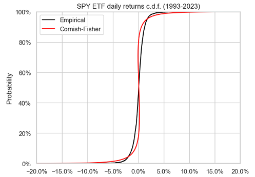
On this figure, it is visible that the Cornish-Fisher distribution does not accurately approximate the empirical distribution of the SPY ETF returns.

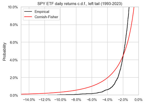
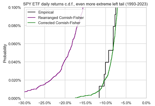
The same also applies to the left tail of the empirical distribution of the SPY ETF returns, as can be seen in Figure 2.

Figure 2. SPY ETF daily returns, empirical c.d.f. v.s. Cornish-Fisher c.d.f., left tail, 1993-2023.

On top of this poor approximation accuracy, and maybe even worse, taking a closer look at Figure 1 also reveals that the Cornish-Fisher distribution does not seem to be monotonous. For example, quantiles between 20% and 40% are positive while quantiles between 60% and 80% are negative! This means that the Cornish-Fisher distribution is not a proper probability distribution¹⁵.

What could explain these observations, while the Cornish-Fisher expansion is supposed, by construction, to be able to approximate the quantiles of any distribution?

Let’s dig in Maillard⁶!

The domain of validity of the Cornish-Fisher expansion

Maillard⁶ notes that in order for the Cornish-Fisher expansion to result in a well-defined quantile function, the skewness parameter $\kappa$ and the excess kurtosis parameter $\gamma$ must satisfy the constraints

\[| \kappa | \leq 6 \left( \sqrt{2} - 1 \right)\] \[27 \gamma^2 - (216 + 66 \kappa^2) \gamma + 40 \kappa^4 + 336 \kappa^2 \leq 0\]

These two constraints define the domain of validity of the Cornish-Fisher expansion, represented in Figure 3.

Figure 3. Domain of validity of the Cornish-Fisher expansion.

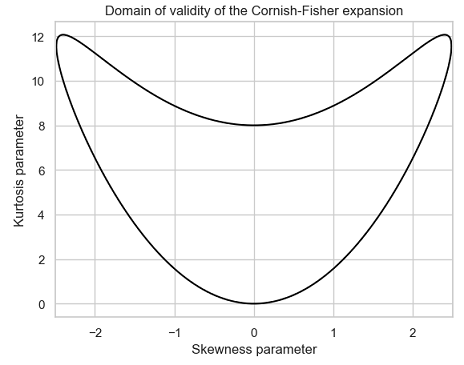
When used outside of its domain of validity, the Cornish-Fisher expansion is known to have several issues impacting its accuracy¹⁶, among which non-monotonous quantiles.

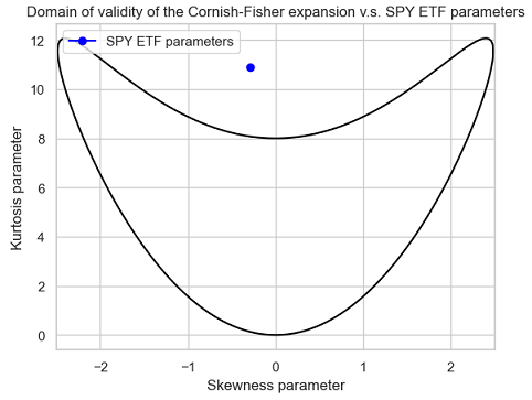
And as can be seen in Figure 4, this is exactly what happens in the case of the SPY ETF, with the parameters $\left( \kappa, \gamma \right) \approx (-0.28740, 10.898897) $ clearly outside of the domain of validity of the Cornish-Fisher expansion.

Figure 4. Domain of validity of the Cornish-Fisher expansion v.s. SPY ETF parameters $\left( \kappa, \gamma \right)$.

Hopefully, there is a way to circumvent the relative narrowness of the domain of validity of the Cornish-Fisher expansion thanks to a regularization procedure called increasing rearrangement¹⁷ and described in details in Chernozhukov et al.¹⁸

The impact of this procedure is illustrated in Figure 5, which compares the same two distributions as in Figure 1, except that the Cornish-Fisher distribution has been rearranged.

Figure 5. SPY ETF daily returns, empirical c.d.f. v.s. rearranged Cornish-Fisher c.d.f., 1993-2023.

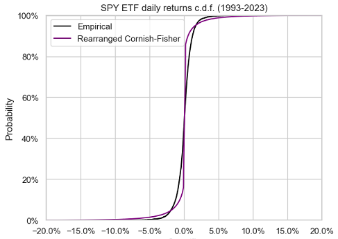
The rearranged Cornish-Fisher distribution is now monotonous, as it should be, but unfortunately, it only marginally better approximates the empirical distribution of the SPY ETF returns.

So, either all hope is lost w.r.t. using mVaR with moderately non-normal return distributions or there is another problem hidden somewhere waiting to be found…

Let’s dig a little bit further in Maillard⁶!

Cornish-Fisher parameters v.s. actual moments

Maillard⁶ also notes that the scale, skewness and excess kurtosis parameters $\sigma$, $\kappa$ and $\gamma$ do not match the actual standard deviation $\sigma_{CF}$, skewness $ \kappa_{CF}$ and excess kurtosis $\gamma_{CF}$ of the Cornish-Fisher distribution $\mathcal{CF}_{\mu, \sigma, \kappa, \gamma}$.

More precisely, he establishes the following relationships

\[\begin{align} \mu_{CF} &= \mu \\ \sigma_{CF} &= \sigma \sqrt{ 1 + \frac{1}{96} \gamma^2 + \frac{25}{1296} \kappa^4 - \frac{1}{36} \gamma \kappa^2 } \\ \kappa_{CF} &= f_1(\kappa, \gamma) \\ \gamma_{CF} &= f_2(\kappa, \gamma) \\ \end{align}\]

, where:

• $\mu_{CF}$, $\sigma_{CF}$, $ \kappa_{CF}$ and $\gamma_{CF}$ are the actual mean, standard deviation, skewness and excess kurtosis of the Cornish-Fisher distribution $\mathcal{CF}_{\mu, \sigma, \kappa, \gamma}$
• $\mu$, $\sigma$, $ \kappa$ and $\gamma$ are the location, scale, skewness and excess kurtosis parameters of the Cornish-Fisher distribution $\mathcal{CF}_{\mu, \sigma, \kappa, \gamma}$
• $f_1$ and $f_2$ are non linear functions, whose explicit formulas are provided in Maillard⁶

As a consequence, when the sample moments of a return distribution are used as plug-in estimators for the Cornish-Fisher parameters, the actual moments of the resulting Cornish-Fisher distribution differ from these sample moments!

Do they differ enough to create a real problem, though?

Re-using the SPY ETF example:

• The sample moments of the SPY ETF empirical return distribution are:
  • $\mu_s \approx 0.000367$
  • $\sigma_s \approx 0.011921$
  • $\kappa_s \approx -0.287409$
  • $\gamma_s \approx 10.898897$
• The actual moments of the Cornish-Fisher distribution $\mathcal{CF}_{\mu_s, \sigma_s, \kappa_s, \gamma_s}$, computed with Maillard’s relationships (1)-(4), are:
  • $\mu_{CF} = \mu_s \approx 0.000367$
  • $\sigma_{CF} \approx 0.017732$
  • $\kappa_{CF} \approx −0.639885$
  • $\gamma_{CF} \approx 62.437532$

So, yes, they do differ a lot, especially the excess kurtosis!

This subtlety is the hidden problem explaining¹⁹ the observed lack of accuracy of modified Value-at-Risk when return distributions are not close to normal⁵. Indeed, it cannot be expected from a “wrong” Cornish-Fisher distribution to accurately approximate anything useful.

The solution to this problem consists in inverting the relationships (1)-(4) between the actual moments and the parameters of the Cornish-Fisher distribution $\mathcal{CF}_{\mu, \sigma, \kappa, \gamma}$.

In other words, we need to determine the value of the parameters $\mu$, $\sigma$, $\kappa$ and $\gamma$ of the Cornish-Fisher distribution $\mathcal{CF}_{\mu, \sigma, \kappa, \gamma}$ so that its actual moments $\mu_{CF}$, $\sigma_{CF}$, $\kappa_{CF}$ and $\gamma_{CF}$ are equal to the sample moments $\mu_{s}$, $\sigma_{s}$, $\kappa_{s}$ and $\gamma_{s}$ of the empirical return distribution, c.f. Lamb et al.⁷.

More on how to do this numerically later.

The resulting Cornish-Fisher distribution is called the corrected Cornish-Fisher distribution $\mathcal{cCF}_{\mu_s, \sigma_s, \kappa_s, \gamma_s}$ and the underlying Cornish-Fisher expansion the corrected Cornish-Fisher expansion⁴.

Re-using one last time the SPY ETF example, we have:

• $\mu \approx 0.000367$
• $\sigma \approx 0.011217$
• $\kappa \approx -0.152059$
• $\gamma \approx 3.556476$

, and Figure 6 compares the resulting corrected Cornish-Fisher distribution to the two distributions of Figure 5.

Figure 6. SPY ETF daily returns, empirical c.d.f. v.s. rearranged Cornish-Fisher c.d.f. and corrected Cornish-Fisher c.d.f., 1993-2023.

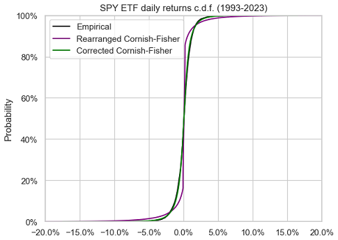
The approximation of the empirical return distribution by the corrected Cornish-Fisher distribution is so accurate that these two distributions are nearly indistinguishable in this figure.

Figure 7, Figure 8 and Figure 9 compare the left tail of the three distributions from Figure 6.

Figure 7. SPY ETF daily returns, empirical c.d.f. v.s. rearranged Cornish-Fisher c.d.f. and corrected Cornish-Fisher c.d.f., left tail, 1993-2023.

Figure 8. SPY ETF daily returns, empirical c.d.f. v.s. rearranged Cornish-Fisher c.d.f. and corrected Cornish-Fisher c.d.f., extreme left tail, 1993-2023.

Figure 9. SPY ETF daily returns, empirical c.d.f. v.s. rearranged Cornish-Fisher c.d.f. and corrected Cornish-Fisher c.d.f., even more extreme left tail, 1993-2023.

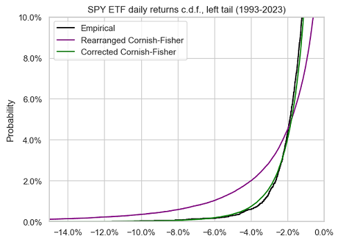
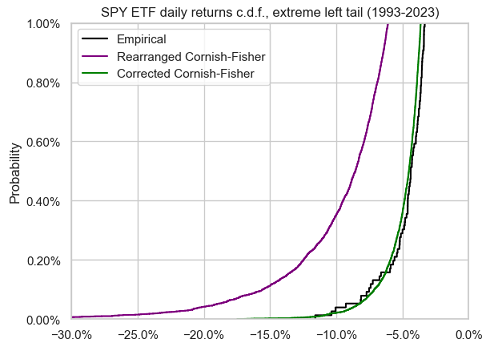
A nearly perfect fit again between the empirical return distribution and the corrected Cornish-Fisher distribution.

This example empirically demonstrates that modified Value-at-Risk, when corrected using Maillard⁶ results, works well for moderately non-normal distributions and for very small tail probabilities.

Computing the corrected Cornish-Fisher distribution

As mentioned in the previous section, computing the corrected Cornish-Fisher distribution requires to invert the relationships (1)-(4) between the actual moments and the parameters of the Cornish-Fisher distribution $\mathcal{CF}_{\mu, \sigma, \kappa, \gamma}$.

Because the location parameter $\mu$ is invariant by (1), and because the scale parameter $\sigma$ is easily computed thanks to (2) once the skewness parameter $\kappa$ and the excess kurtosis parameter $\gamma$ have been computed, the main mathematical challenge is to invert the system of non-linear equations (3)-(4).

The domain of validity of the corrected Cornish-Fisher expansion

Before thinking about how to invert these equations numerically, we first need to make sure that they are invertible theoretically.

Lamb et al.⁷ prove that this is the case when the actual skewness $\kappa_{CF}$ and the actual excess kurtosis $\gamma_{CF}$ belong²⁰ to what could be called the domain of validity of the corrected Cornish-Fisher expansion²¹, represented in Figure 10.

Figure 10. Domain of validity of the corrected Cornish-Fisher expansion.

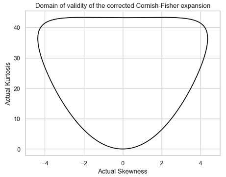
Lamb et al.⁷ also establish that the resulting skewness parameter $\kappa$ and excess kurtosis parameter $\gamma$ belong to the domain of validity of the Cornish-Fisher expansion, which ensures that the resulting corrected Cornish-Fisher distribution is a proper distribution.

To be noted that the domain of validity of the corrected Cornish-Fisher expansion (Figure 10) is much wider than the domain of validity of the Cornish-Fisher expansion (Figure 3).

This is extremely important in applications, because the actual skewness $\kappa_{CF}$ and the actual excess kurtosis $\gamma_{CF}$ of the corrected Cornish-Fisher distribution typically correspond to the sample skewness $\kappa_s$ and to the sample excess kurtosis $\gamma_s$ of a given distribution²², so that the corrected Cornish-Fisher distribution is valid in practice for a much wider range of skewness and excess kurtosis than the non-corrected Cornish-Fisher distribution.

The inversion procedure

At least two algorithms have been analyzed in the literature to compute the corrected Cornish-Fisher parameters from the actual moments:

• A kind of interpolation algorithm, using the response surface methodology, in Amedee-Manesme et al.⁴
• A modified Newton method, in Lamb et al.⁷

Implementation in Portfolio Optimizer

Portfolio Optimizer implements a proprietary algorithm to compute the parameters of the corrected Cornish-Fisher distribution, whose general description is:

• Determine the actual mean $\mu_s$, standard deviation $\sigma_s$, skewness $\kappa_s$ and excess kurtosis $\gamma_s$ of the corrected Cornish-Fisher distribution

  These are either directly provided in input of the endpoint (e.g. /assets/returns/simulation/monte-carlo/cornish-fisher/corrected) or computed from an empirical distribution of returns (e.g. /portfolio/analysis/value-at-risk/cornish-fisher/corrected).

• If the skewness $\kappa_s$ and the excess kurtosis $\gamma_s$ belong to the domain of validity of the corrected Cornish-Fisher expansion, a robust iterative numerical method is then used to compute the skewness and excess kurtosis parameters $\kappa$ and $\gamma$.

  Once these parameters are known, the relationships (1)-(4) allow to determine the resulting corrected Cornish-Fisher distribution $\mathcal{cCF}_{\mu_s, \sigma_s, \kappa_s, \gamma_s}$.

• Otherwise, a robust iterative numerical method is used to tentatively²³ compute the skewness and excess kurtosis parameters $\kappa$ and $\gamma$

  • If this computation is successful, the increasing rearrangement procedure of Chernozhukov et al.¹⁸ is applied to the resulting corrected Cornish-Fisher distribution $\mathcal{cCF}_{\mu_s, \sigma_s, \kappa_s, \gamma_s}$ in order to transform it into a valid distribution
  • Otherwise, an error is raised

Example of usage - Computing the modified Value-at-Risk of Bitcoin

Bitcoin is an example of asset exhibiting strong non-normal characteristics²⁴, for which the standard measures of Value-at-Risk like Gaussian Value-at-Risk or modified Value-at-Risk would be inaccurate.

But what about modified Value-at-Risk based on the corrected Cornish-Fisher expansion?

In order to investigate the accuracy of this measure, that I will call corrected Cornish-Fisher Value-at-Risk (cCFVaR), Figure 11 compares, over the period 20 August 2011 - 06 April 2023, the empirical distribution of Bitcoin daily returns¹⁴ to the corrected Cornish-Fisher distribution $\mathcal{cCF}_{\mu_s, \sigma_s, \kappa_s, \gamma_s}$ with actual moments:

• $\mu_s \approx 0.001863$, the sample mean of Bitcoin returns over the considered period
• $\sigma_s \approx 0.047369$, the sample standard deviation of Bitcoin returns over the considered period
• $\kappa_s \approx -1.368879$, the sample skewness of Bitcoin returns over the considered period
• $\gamma_s \approx 24.594523$, the sample excess kurtosis of Bitcoin returns over the considered period

Figure 11. Bitcoin daily returns, empirical c.d.f. v.s. corrected Cornish-Fisher c.d.f., 2011-2023.

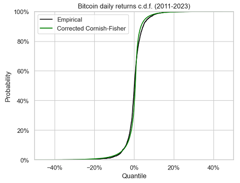
It seems that the corrected Cornish-Fisher distribution does a pretty good job in approximating the empirical return distribution of Bitcoin, except in the right tail though.

Figure 12 and Figure 13 compare the left tail of these two distributions.

Figure 12. Bitcoin daily returns, empirical c.d.f. v.s. corrected Cornish-Fisher c.d.f., left tail, 2011-2023.

Figure 13. Bitcoin daily returns, empirical c.d.f. v.s. corrected Cornish-Fisher c.d.f., extreme left tail, 2011-2023.

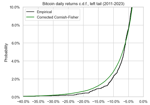
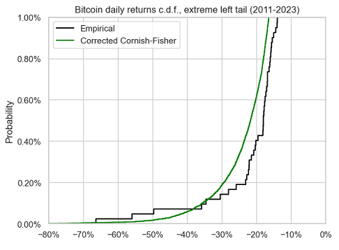
There figures confirm that the corrected Cornish-Fisher distribution accurately approximates the empirical return distribution of Bitcoin down to a confidence level of $\approx 95\%$, but no lower.

This can also be confirmed numerically, with a comparison between historical Value-at-Risk and corrected Cornish-Fisher Value-at-Risk at different confidence levels:

Confidence level $\alpha$	$\text{HVaR}_{\alpha}$	$\text{cCFVaR}_{\alpha}$
95%	6.90%	6.86%
97.5%	9.53%	10.63%
99%	13.36%	16.51%
99.5%	15.92%	21.56%
99.9%	27.04%	35.08%

All in all, this example empirically demonstrates that modified Value-at-Risk, when corrected following Maillard⁶ results, works well for highly non-normal distributions with not too small tail probabilities.

Conclusion

The goal of this post was to highlight that accuracy issues reported by practitioners with modified Value-at-Risk have been understood since more than ten years, but that, as Amedee-Manesme et al.⁴ put it:

this point […] does not seem to have received sufficient attention

If you are such a practitioner, I hope that this post will encourage you to double check how modified Value-at-Risk is computed by your internal risk management software.

Waiting for an answer from your (puzzled) IT teams, feel free to connect with me on LinkedIn or follow me on Twitter.

–

1. See Zangari, P. (1996). A VaR methodology for portfolios that include options. RiskMetrics Monitor First Quarter, 4–12. ↩ ↩²

2. See Martin, R. Douglas and Arora, Rohit, Inefficiency of Modified VaR and ES. ↩ ↩² ↩³ ↩⁴

3. For example, European financial regulators require to use mVaR in order to compute the Summary Risk Indicator (SRI), i.e. the risk score, of Packaged Retail Investment and Insurance Products (PRIIPs) starting 1st January 2023, c.f. regulatory Technical Standards on the content and presentation of the KIDs for PRIIPs. ↩

4. See Amedee-Manesme, CO., Barthelemy, F. & Maillard, D. Computation of the corrected Cornish–Fisher expansion using the response surface methodology: application to VaR and CVaR. Ann Oper Res 281, 423–453 (2019). ↩ ↩² ↩³ ↩⁴

5. See Stoyan V. Stoyanov, Svetlozar T. Rachev, Frank J. Fabozzi, Sensitivity of portfolio VaR and CVaR to portfolio return characteristics, Working paper. ↩ ↩² ↩³

6. See Maillard, Didier, A User’s Guide to the Cornish Fisher Expansion. ↩ ↩² ↩³ ↩⁴ ↩⁵ ↩⁶ ↩⁷ ↩⁸ ↩⁹

7. See Lamb, John D., Maura E. Monville, and Kai-Hong Tee. Making Cornish–fisher Fit for Risk Measurement, Journal of Risk, Volume 21, Number 5, Pages 53-81. ↩ ↩² ↩³ ↩⁴ ↩⁵ ↩⁶ ↩⁷

8. Like 1% quantile or even less. ↩

9. See Jorion, P. (2007). Value at risk: The new benchmark for managing financial risk. New York, NY: McGraw-Hill. ↩

10. In this post, returns are assumed to be logarithmic returns. ↩

11. This is the case when the portfolio return cumulative distribution function is strictly increasing and continuous; otherwise, a similar formula is still valid, with $F_X^{-1}$ the generalized inverse distribution function of $X$, but these subtleties - important in mathematical proofs and in numerical implementations - are out of scope of this post. ↩

12. See Boudt, Kris and Peterson, Brian G. and Croux, Christophe, Estimation and Decomposition of Downside Risk for Portfolios with Non-Normal Returns (October 31, 2007). Journal of Risk, Vol. 11, No. 2, pp. 79-103, 2008. ↩ ↩²

13. Asset returns have a tendency to follow a distribution closer and closer to a Gaussian distribution the more the time period over which they are computed increases; this empirical property is called aggregational Gaussianity, c.f. Cont²⁵. ↩

14. The associated adjusted prices have been retrieved using Tiingo. ↩ ↩²

15. This also means that it is possible to have $\text{mVaR}_{95\%} > \text{mVaR}_{99\%} $, which requires some funny arguments to be explained… ↩

16. See Barton, D.E., & Dennis, K.E. (1952). The conditions under which Gram-Charlier and Edgeworth curves are positive definite and unimodal. Biometrika, 39(3-4), 425–427. ↩

17. I will not enter into the mathematical details in this post, but it suffices to say that this procedure allows to correct the behavior of the Cornish-Fisher expansion when used outside of its domain of validity thanks to a sorting operator. ↩

18. See Chernozhukov, V., Fernandez-Val, I. & Galichon, A. Rearranging Edgeworth–Cornish–Fisher expansions. Econ Theory 42, 419–435 (2010). ↩ ↩²

19. In addition, Maillard⁶ mentions that when the skewness and excess kurtosis parameters are small enough, in a loose sense, they coincide with the actual skewness and excess kurtosis of the Cornish-Fisher distribution, which perfectly explains the behavior of the modified Value-at-Risk observed in practice with return distributions close to normal⁵. ↩

20. Actually, the result of Lamb et al.⁷ is a little bit more generic: they establish that the system of non-linear equations is invertible on a region which includes the domain of validity of the Cornish-Fisher expansion. ↩

21. The domain of validity of the corrected Cornish-Fisher expansion is the mathematical image, by the functions $f_1$ and $f_2$, of the domain of validity of the Cornish-Fisher expansion. ↩

22. In the context of this blog post, the given distribution is a return distribution (asset, portfolio, strategy…). ↩

23. This tentative computation is theoretically justified by the results from Lamb et al.⁷. ↩

24. See Joerg Osterrieder, The Statistics of Bitcoin and Cryptocurrencies, Proceedings of the 2017 International Conference on Economics, Finance and Statistics (ICEFS 2017). ↩

25. See R. Cont (2001) Empirical properties of asset returns: stylized facts and statistical issues, Quantitative Finance, 1:2, 223-236. ↩