Volatility Forecasting: HExp Model

In this series on volatility forecasting, I previously detailed the Heterogeneous AutoRegressive (HAR) volatility forecasting model that has become the workhorse of the volatility forecasting literature¹ since its introduction by Corsi².

I will now describe an extension of that model due to Bollerslev et al.³, called the Heterogeneous Exponential (HExp) volatility forecasting model, in which the lagged HAR volatility components are exponentially - rather than arithmetically - averaged.

In addition, I will also discuss the panel-based estimation procedure for the HExp and the HAR model parameters proposed in Bollerslev et al.³, which is empirically demonstrated³ to improve the out-of-sample forecasting performances of these two volatility forecasting models when compared to the standard² individual asset-based procedure.

Finally, I will illustrate the practical performances of the HExp volatility forecasting model and its panel-based parameters estimation procedure in the context of monthly volatility forecasting for various ETFs.

Mathematical preliminaries (reminders)

This section contains reminders from the first blog post of this series.

Volatility modelling and volatility proxies

Let $r_t$ be the logarithmic return of an asset over a time period $t$ (a day, a week, a month..), over which its (conditional) mean return is supposed to be null.

Then:

• The asset (conditional) variance is defined as $ \sigma_t^2 = \mathbb{E} \left[ r_t^2 \right] $

  From this definition, the squared return $r_t^2$ of an asset is a (noisy⁴) variance estimator - or variance proxy⁴ - for that asset variance over the considered time period.

  Another example of an asset variance proxy is the Parkinson range of an asset.

  Yet another example of an asset variance proxy, this time over a specific time period $t$ of one day, is the daily realized variance $RV_t$, which is defined as the sum of the asset squared intraday returns sampled at a high frequency (1 minutes, 5 minutes, 15 minutes…).

  The generic notation for an asset variance proxy in this blog post is $\tilde{\sigma}_t^2$.

• The asset (conditional) volatility is defined as $ \sigma_t = \sqrt { \sigma_t^2 } $

  The generic notation for an asset volatility proxy in this blog post is $\tilde{\sigma}_t$.

Weighted moving average volatility forecasting model

Boudoukh et al.⁵ shows that many seemingly different methods of volatility forecasting actually share the same underlying representation of the estimate of an asset next period’s variance $\hat{\sigma}_{T+1}^2$ as a weighted moving average of that asset past periods’ variance proxies $\tilde{\sigma}^2_t$, $t=1..T$, with

\[\hat{\sigma}_{T+1}^2 = w_0 + \sum_{i=1}^{k} w_i \tilde{\sigma}^2_{T+1-i}\]

, where:

• $k$, with $1 \leq k \leq T$, is the size of the moving average, possibly time-dependent
• $w_i, i=0..k$ are the weights of the moving average, possibly time-dependent as well

The original HAR volatility forecasting model

The HAR volatility forecasting model is an additive cascade model of different volatility components² subject to economically meaningful restrictions².

Under that model, an asset next day’s daily realized variance $RV_{T+1}$ is forecasted through the formula⁴:

\[\hat{RV}_{T+1} = \beta + \beta_d RV_{T} + \beta_w RV_{T}^w + \beta_m RV_{T}^m\]

, where:

• $\hat{RV}_{T+1}$ is the forecast at time $T$ of the asset next day’s daily realized variance $RV_{T+1}$
• $RV_T$ is the asset daily realized variance at time $T$
• $RV_T^w = \frac{1}{5} \sum_{i=1}^5 RV_{T-i+1}$ is the asset weekly realized variance at time $T$
• $RV_T^m = \frac{1}{22} \sum_{i=1}^{22} RV_{T-i+1}$ is the asset monthly realized variance at time $T$
• $\beta$, $\beta_d$, $\beta_w$ and $\beta_m$ are the HAR model parameters, to be determined

The HExp volatility forecasting model

Discontinuity of the HAR volatility forecasting model

Under the HAR volatility forecasting model, forecasted future volatilities depends on the past volatilities in a way that is [dis]continuous […] in the lag lengths³ due to the presence of simple moving averages, which might lead to potential variance estimation issues³.

As noted by Bollerslev et al.³:

The stepwise nature of the volatility factors employed in the HAR models, imply that the forecasts from the models are subject to potentially abrupt changes as an unusually large/small daily lagged [realized variance] drops out of the sums for the longer-horizon lagged volatility factors.

Figure 1, adapted from Bollerslev et al.³, illustrates the lag coefficients implied by the regression coefficients³ of the HAR model together with those of a 21-day simple moving average model.

Figure 1. Lag coefficients of the HAR and of the 21-day simple moving average volatility forecasting models. Source: Bollerslev et al.

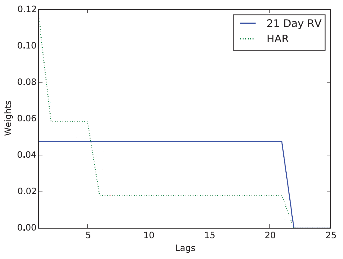
The discontinuity of the HAR model at the 1-day, 5-day and 21-day lags⁶ is apparent, similar in spirit to the discontinuity of the 21-day simple moving average model at the 21-day lag.

The original HExp volatility forecasting model

In order to avoid the stepwise changes inherent in the forecast from the HAR component-type structure³, Bollerslev et al.³ proposes to replace the simple moving averages appearing in the HAR model by exponentially weighted moving averages.

Under the resulting volatility forecasting model - denoted the Heterogenous Exponential realized volatility model (HExp for short)³ - an asset next day’s daily realized variance $RV_{T+1}$ is forecasted through the formula³⁷

\[\hat{RV}_{T+1} = \beta + \beta_d ExpVP_T^{\lambda(1)} + \beta_w ExpVP_T^{\lambda(5)} + \beta_m ExpVP_T^{\lambda(25)} + \beta_h ExpVP_T^{\lambda(125)}\]

, where:

• $\hat{RV}_{T+1}$ is the forecast at time $T$ of the asset next day’s daily realized variance $RV_{T+1}$
• $ExpVP_T^{\lambda(CoM)}$ $=$ $\sum_{i=1}^T \frac{e^{-i \lambda(CoM)}}{\sum_{j=1}^T e^{-j \lambda(CoM)}} RV_{T+1-i} $
• $\lambda \left(CoM\right)$ $=$ $\log \left( 1 + \frac{1}{CoM} \right)$, with CoM standing for center-of-mass³
• $RV_i$ is the asset daily realized variance at time $i$, $i=1..T$
• $\beta$, $\beta_d$, $\beta_w$, $\beta_m$ and $\beta_h$ are the HExp model parameters, to be determined

To be noted that each center-of-mass used in the HExp model (1, 5, 25 and 125) effectively summarizes the “average” horizon of the lagged realized volatilities that it uses³ and that they all have been chosen in Bollerslev et al.³ so as to “span” the universe of past [realized variance]’s in a way that is both parsimonious and “smooth”³.

Speaking of smoothness, Figure 2, again adapted from Bollerslev et al.³, compares the lag coefficients implied by the regression coefficients³ of the HAR model with those of the HExp model.

Figure 2. Lag coefficients of the HAR and of the HExp volatility forecasting models. Source: Bollerslev et al.

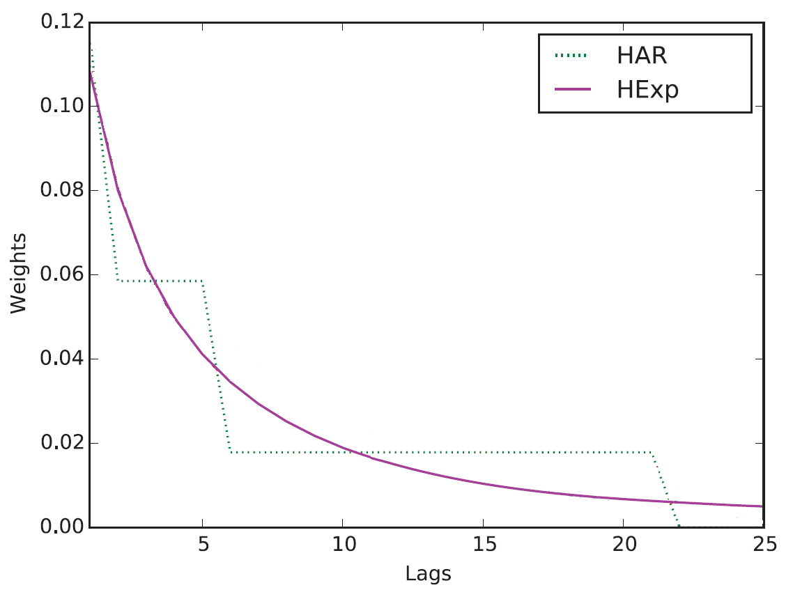
The continuous nature of the HExp volatility forecasting model is clearly visible.

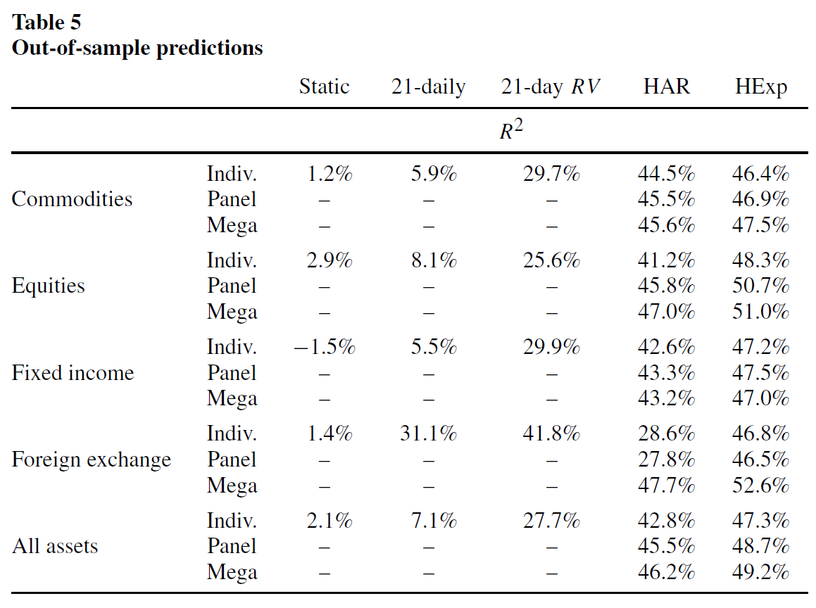
In terms of practical performances, the HExp model perform[s] well in out-of-sample risk forecasting³ and is even slightly more performant than the HAR model in terms of $r$-squared, as can be seen on Figure 3 adapted from Bollerslev et al.³.

Figure 3. Out-of-sample $r$-squared of the HAR model v.s. the HExp model for predicting the 20-day future realized volatility of several assets and for different methods of parameters estimation (Ind, Panel, Mega, that will be discussed in the next section). Source: Bollerslev et al.

Realized variance v.s. generic variance proxy

The original HExp model described in the previous subsection relies on a very specific asset variance proxy - the realized variance of an asset - over a very specific time period - a day - for its definition.

Similarly to the HAR model, it is possible to replace the daily realized variance by any generic daily variance estimator like daily squared returns⁸ or any daily range-based variance estimator (Parkinson, Garman-Klass, Rogers-Satchell…).

This leads to the generic HExp volatility forecasting model, under which an asset next days’s conditional variance $\sigma_{T+1}^2$ is forecasted through the formula

\[\hat{\sigma}_{T+1}^2 = \beta + \beta_d ExpVP_T^{\lambda(1)} + \beta_w ExpVP_T^{\lambda(5)} + \beta_m ExpVP_T^{\lambda(25)} + \beta_h ExpVP_T^{\lambda(125)}\]

, where:

• $\hat{\sigma}_{T+1}^2$ is the forecast at time $T$ of the asset next day’s conditional variance $\sigma_{T+1}^2$
• $ExpVP_T^{\lambda(CoM)} = \sum_{i=1}^T \frac{e^{-i \lambda(CoM)}}{\sum_{j=1}^T e^{-j \lambda(CoM)}} \tilde{\sigma}^2_{T+1-i} $
• $\lambda \left(CoM\right) = \log \left( 1 + \frac{1}{CoM} \right) $
• $\tilde{\sigma}^2_{i}$ is the asset daily variance estimator at time $i$, $i=1..T$
• $\beta$, $\beta_d$, $\beta_w$, $\beta_m$ and $\beta_h$ are the HExp model parameters, to be determined

Relationship with the generic weighted moving average model

From its definition, it is not too difficult to see that the HExp volatility forecasting model is a specific kind of weighted moving average volatility forecasting model, with:

• $w_0 = \beta$
• $w_1 = \beta_d \frac{e^{- \lambda(1)}}{\sum_{j=1}^T e^{-j \lambda(1)}}$ $+$ $\beta_w \frac{e^{- \lambda(5)}}{\sum_{j=1}^T e^{-j \lambda(5)}}$ $+$ $\beta_m \frac{e^{- \lambda(25)}}{\sum_{j=1}^T e^{-j \lambda(25)}}$ $+$ $\beta_h \frac{e^{- \lambda(125)}}{\sum_{j=1}^T e^{-j \lambda(125)}} $
• $w_2 = …$

Volatility forecasting formulas

Under an HExp volatility forecasting model, the generic weighted moving average volatility forecasting formula becomes:

• To estimate an asset next day’s volatility:

  \[\hat{\sigma}_{T+1} = \sqrt{ \beta + \beta_d ExpVP_T^{\lambda(1)} + \beta_w ExpVP_T^{\lambda(5)} + \beta_m ExpVP_T^{\lambda(25)} + \beta_h ExpVP_T^{\lambda(125)} }\]

• To estimate an asset next $h$-day’s ahead volatility⁹, $h \geq 2$, using an indirect¹ multi-step ahead forecast scheme:

  \[\hat{\sigma}_{T+h} = \sqrt{ \beta + \beta_d ExpVP_{T+h-1}^{\lambda(1)} + \beta_w ExpVP_{T+h-1}^{\lambda(5)} + \beta_m ExpVP_{T+h-1}^{\lambda(25)} + \beta_h ExpVP_{T+h-1}^{\lambda(125)} }\]

, where:

• $ExpVP_{T+h-1}^{\lambda(CoM)}$ $=$ $\sum_{i=1}^T \frac{e^{-i \lambda(CoM)}}{\sum_{j=1}^{T+h-1} e^{-j \lambda(CoM)}} \tilde{\sigma}^2_{T+1-i} $ $+$ $\sum_{i=1}^{h-1} \frac{e^{-i \lambda(CoM)}}{\sum_{j=1}^{T+h-1} e^{-j \lambda(CoM)}} \hat{\sigma}^2_{T+h-i} $

• To estimate an asset aggregated volatility⁹ over the next $h$ days:

  \[\hat{\sigma}_{T+1:T+h} = \sqrt{ \sum_{i=1}^{h} \hat{\sigma}^2_{T+i} }\]

Estimating the HExp model parameters

Individual estimation

As for the HAR model, the easiest way to estimate the HExp model parameters is by applying simple linear regression² on an asset-by-asset basis³, in which case the asset-specific ordinary least squares (OLS) estimator of the parameters $\beta$, $\beta_d$, $\beta_w$, $\beta_m$ and $\beta_h$ at time $T$ is the solution of the minimization problem⁴

\[\argmin_{ \left( \beta, \beta_d, \beta_w, \beta_m, \beta_h \right) \in \mathbb{R}^{5}} \sum_{t=1}^T \left( \tilde{\sigma}_{t}^2 - \beta - \beta_d ExpVP_{t-1}^{\lambda(1)} - \beta_w ExpVP_{t-1}^{\lambda(5)} - \beta_m ExpVP_{t-1}^{\lambda(25)} - \beta_h ExpVP_{t-1}^{\lambda(125)} \right)^2\]

Alternatively, following Clements and Preve⁴ and Clements et al.¹, more complex asset-specific least squares estimators than OLS can be used to try to improve forecast performances (weighted least squares estimators (WLS), robust least squares estimators (RLS)…)

Panel-based estimation

Bollerslev et al.³ establishes that the dynamics of realized volatility are common across many different financial assets.

This is illustrated in Figure 4, directly taken from Bollerslev et al.³, which depicts the unconditional distributions of daily normalized realized volatilities for different asset classes.

Figure 4. Normalized unconditional daily realized variance distributions for misc. asset classes. Source: Bollerslev et al.

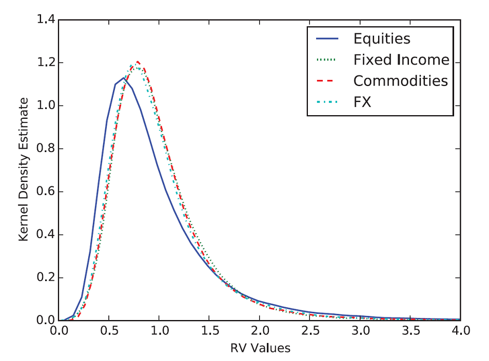
From this figure, volatility indeed seems to behave similarly across asset classes³ and Bollerslev et al.³ proposes to exploit these strong similarities in the distributions of the volatilities across and within asset classes³ by using panel regression techniques that force the [HExp model parameters] to be the same within and across different asset classes³.

In more details, Bollerslev et al.³ reformulates the generic HExp volatility forecasting model as follows:

\[\hat{\sigma}_{T+1}^2 = \tilde{\sigma}_{T}^{2, LR} + \beta_d^P \left( ExpVP_T^{\lambda(1)} - \tilde{\sigma}_{T}^{2, LR} \right) + \beta_w^P \left( ExpVP_T^{\lambda(5)} - \tilde{\sigma}_{T}^{2, LR} \right) + \beta_m^P \left( ExpVP_T^{\lambda(25)} - \tilde{\sigma}_{T}^{2, LR} \right) + \beta_h^P \left( ExpVP_T^{\lambda(125)} - \tilde{\sigma}_{T}^{2, LR} \right)\]

, where:

• $ \tilde{\sigma}_{T}^{2, LR}$ is a long-run volatility factor, equal to the expanding sample mean of [the asset daily variance estimator] from the start of the sample up until day $T$³.
• $\beta_d^P$, $\beta_w^P$, $\beta_m^P$ and $\beta_h^P$ are the HExp “panel” model parameters, to be determined

Such a reformulation - called centering³ in Bollerslev et al.³ - eliminat[es] the level of the [asset] volatility³ from the HExp model and enables¹⁰ the parameters $\beta_d^P$, $\beta_w^P$, $\beta_m^P$ and $\beta_h^P$ to be estimated simultaneously for all assets by panel regression techniques that add power by exploiting the similarities in the cross-asset risk characteristics³.

Additionally¹¹, that specific reformulation ensures that the iterated long-run forecasts from the model constructed on day $T$ converges to this day $T$ estimate of the “unconditional” volatility³.

From a practical perspective, Figure 3 shows that estimating the HExp parameters¹² through panel-based estimation (lines Panel and Mega) leads to much better performances v.s. their individual estimation (lines Ind).

Implementation in Portfolio Optimizer

Portfolio Optimizer implements the HExp volatility forecasting model - together with all the extensions of its predecessor (the insanity filter described in Clements and Preve⁴, the log transformation…) - through the endpoint /assets/volatility/forecast/hexp.

This endpoint supports the 4 variance proxies below:

• Squared close-to-close returns
• Demeaned squared close-to-close returns
• The Parkinson range
• The jump-adjusted Parkinson range

This endpoint also supports:

• Individual and panel-based estimation of the HExp model parameters.

• Using up to 5 centers-of-mass for the variance proxies, the default ones being 1, 5 and 25¹³.

Example of usage - Volatility forecasting at monthly level for various ETFs

As an example of usage, I propose to enrich the results of the previous blog post, in which monthly forecasts produced by different volatility models¹⁴ are compared - using Mincer-Zarnowitz¹⁵ regressions - to the next month’s close-to-close observed volatility for 10 ETFs representative¹⁶ of misc. asset classes:

• U.S. stocks (SPY ETF)
• European stocks (EZU ETF)
• Japanese stocks (EWJ ETF)
• Emerging markets stocks (EEM ETF)
• U.S. REITs (VNQ ETF)
• International REITs (RWX ETF)
• U.S. 7-10 year Treasuries (IEF ETF)
• U.S. 20+ year Treasuries (TLT ETF)
• Commodities (DBC ETF)
• Gold (GLD ETF)

Individual estimation

Averaged results for all ETFs/regression models over each ETF price history¹⁷ are the following¹⁸, when adding the HExp volatility forecasting model and its log variation¹⁹:

Volatility model	Variance proxy	$\bar{\alpha}$	$\bar{\beta}$	$\bar{R^2}$
EWMA, optimal $\lambda$	Squared close-to-close returns	4.7%	0.73	45%
HAR	Squared close-to-close returns	-0.7%	0.95	46%
HAR (log)	Squared close-to-close returns	0.5%	0.62	40%
HExp	Squared close-to-close returns	-0.7%	0.93	48%
HExp (log)	Squared close-to-close returns	2.1%	0.57	42%
EWMA, optimal $\lambda$	Parkinson range	4.3%	1.06	48%
HAR	Parkinson range	0.1%	1.25	44%
HAR (log)	Parkinson range	1.9%	1.22	50%
HExp	Parkinson range	-0.5%	1.29	47%
HExp (log)	Parkinson range	2.0%	1.21	51%
EWMA, optimal $\lambda$	Jump-adjusted Parkinson range	4.0%	0.76	45%
HAR	Jump-adjusted Parkinson range	-1.4%	0.99	47%
HAR (log)	Jump-adjusted Parkinson range	0.9%	0.92	51%
HExp	Jump-adjusted Parkinson range	-1.5%	0.98	49%
HExp (log)	Jump-adjusted Parkinson range	1.1%	0.91	52%

Panel-based estimation

Averaged results for all ETFs/regression models over the common ETF price history²⁰ are the following¹⁸:

• When using the EWMA, HAR and HExp volatility forecasting models with an asset-specific parameters estimation procedure (for reference):

  Volatility model	Variance proxy	$\bar{\alpha}$	$\bar{\beta}$	$\bar{R^2}$
  EWMA, optimal $\lambda$ (individual est.)	Squared close-to-close returns	5%	0.72	43%
  HAR (individual est.)	Squared close-to-close returns	-0.2%	0.89	46%
  HExp (individual est.)	Squared close-to-close returns	0.02%	0.87	47%
  EWMA, optimal $\lambda$ (individual est.)	Parkinson range	4.8%	1.02	45%
  HAR (individual est.)	Parkinson range	0.7%	1.17	46%
  HExp (individual est.)	Parkinson range	1.2%	1.15	47%
  EWMA, optimal $\lambda$ (individual est.)	Jump-adjusted Parkinson range	4.5%	0.73	43%
  HAR (individual est.)	Jump-adjusted Parkinson range	-0.9%	0.94	46%
  HExp (individual est.)	Jump-adjusted Parkinson range	-0.4%	0.90	46%

• When using the HAR and HExp volatility forecasting models with a panel-based parameters estimation procedure comparable to the Mega procedure described in Bollerslev et al.³:

  Volatility model	Variance proxy	$\bar{\alpha}$	$\bar{\beta}$	$\bar{R^2}$
  HAR (panel est.)	Squared close-to-close returns	2.2%	0.76	47%
  HExp (panel est.)	Squared close-to-close returns	1.1%	0.80	47%
  HAR (panel est.)	Parkinson range	3.1%	1.11	50%
  HExp (panel est.)	Parkinson range	3.6%	1.08	50%
  HAR (panel est.)	Jump-adjusted Parkinson range	0.09%	0.88	46%
  HExp (panel est.)	Jump-adjusted Parkinson range	-0.07%	0.89	48%

Comments

From the results of the two previous subsections, it is possible to make the following comments:

• Consistent with Bollerslev et al.³, the HExp model is uniformly better than the HAR model in terms of r-squared.

• Contrary to Bollerslev et al.³, the panel-based estimation procedure does not seem to dramatically improve the HAR/HExp models performances, except when the Parkinson range is used as a daily variance proxy.

  Comparing lines #1,2,5,6 with lines #3,4 suggests to perform the same test with (high frequency) realized variances in order to confirm that this is due to the “quality” of the daily variance proxy used.

Conclusion

This blog post empirically confirmed that the HExp volatility forecasting model of Bollerslev et al.³ belongs to the category of the state-of-the-art dynamic [risk models]³ published in the litterature.

This blog post also concludes this series on volatility forecasting by weighted moving average models, at least until I find a better such model than the HExp model.

Waiting for that to happen or for a blog post on volatility forecasting by a non-weighted moving average model, feel free to connect with me on LinkedIn or to follow me on Twitter.

–

1. See Clements, Adam and Preve, Daniel P. A. and Tee, Clarence, Harvesting the HAR-X Volatility Model. ↩ ↩² ↩³

2. See Fulvio Corsi, A Simple Approximate Long-Memory Model of Realized Volatility, Journal of Financial Econometrics, Volume 7, Issue 2, Spring 2009, Pages 174–196. ↩ ↩² ↩³ ↩⁴ ↩⁵

3. See Tim Bollerslev, Benjamin Hood, John Huss, Lasse Heje Pedersen, Risk Everywhere: Modeling and Managing Volatility, The Review of Financial Studies, Volume 31, Issue 7, July 2018, Pages 2729–2773. ↩ ↩² ↩³ ↩⁴ ↩⁵ ↩⁶ ↩⁷ ↩⁸ ↩⁹ ↩¹⁰ ↩¹¹ ↩¹² ↩¹³ ↩¹⁴ ↩¹⁵ ↩¹⁶ ↩¹⁷ ↩¹⁸ ↩¹⁹ ↩²⁰ ↩²¹ ↩²² ↩²³ ↩²⁴ ↩²⁵ ↩²⁶ ↩²⁷ ↩²⁸ ↩²⁹ ↩³⁰ ↩³¹ ↩³² ↩³³ ↩³⁴ ↩³⁵ ↩³⁶ ↩³⁷ ↩³⁸ ↩³⁹

4. See Adam Clements, Daniel P.A. Preve, A Practical Guide to harnessing the HAR volatility model, Journal of Banking & Finance, Volume 133, 2021. ↩ ↩² ↩³ ↩⁴ ↩⁵ ↩⁶

5. See Boudoukh, J., Richardson, M., & Whitelaw, R.F. (1997). Investigation of a class of volatility estimators, Journal of Derivatives, 4 Spring, 63-71. ↩

6. These lags correspond to the daily, weekly and monthly realized variance components of the original HAR model. ↩

7. In Bollerslev et al.³, the calculation of $ExpVP_T^{\lambda(CoM)}$ uses only the first 500 lags (i.e., is truncated to $T=500$) because the influence of the remaining lags is numerically immaterial³. ↩

8. Bollerslev et al.³ discusses the impact of replacing realized volatilities by daily squared returns in the HExp model. ↩

9. See Brooks, Chris and Persand, Gitanjali (2003) Volatility forecasting for risk management. Journal of Forecasting, 22(1). pp. 1-22. ↩ ↩²

10. Eliminating the level of the asset volatility is a pre-requisite in order to use panel regression techniques because the very different volatility levels for different asset classes means that³ 1) it is unreasonable to force the $\beta$ intercepts to be the same³ for all assets and 2) it is necessary to ensure that all [the remaining] parameters are “scale-free” in the sense that they do not depend on the level of risk³. ↩

11. Thanks to that reformulation, the coefficients $\beta_d$, $\beta_w$, $\beta_m$ and $\beta_h$ are also free (i.e., need not sum to one)³, which allows an easy fitting through OLS. ↩

12. As a side note, the centering reformulation described in Bollerslev et al.³ is also applicable to the HAR volatility forecasting model and is done in Bollerslev et al.³. ↩

13. Contrary to Bollerslev et al.³, the center-of-mass 125 is not included by default in the HExp model as implemented in Portfolio Optimizer; this choice was made to make the default HExp model implementation directly comparable with the default HAR model implementation. ↩

14. Using Portfolio Optimizer. ↩

15. See Mincer, J. and V. Zarnowitz (1969). The evaluation of economic forecasts. In J. Mincer (Ed.), Economic Forecasts and Expectations. ↩

16. These ETFs are used in the Adaptative Asset Allocation strategy from ReSolve Asset Management, described in the paper Adaptive Asset Allocation: A Primer²¹. ↩

17. The common ending price history of all the ETFs is 31 August 2023, but there is no common starting price history, as all ETFs started trading on different dates. ↩

18. For all models, I used an expanding window for the volatility forecast computation. ↩ ↩²

19. The log HExp model is similar in spirit to the log HAR model described in the previous blog post. ↩

20. The common starting price history of the ETFs is 31 July 2007 and their common ending price history is 31 August 2023. ↩

21. See Butler, Adam and Philbrick, Mike and Gordillo, Rodrigo and Varadi, David, Adaptive Asset Allocation: A Primer. ↩