Volatility Forecasting: HAR Model

Among the different members of the family of volatility forecasting models by weighted moving average¹ like the simple and the exponentially weighted moving average models or the GARCH(1,1) model, the Heterogeneous AutoRegressive (HAR) model introduced by Corsi² has become the workhorse of the volatility forecasting literature³ on account of its simplicity and generally good forecasting performance³.

In this blog post, strongly inspired by the paper A Practical Guide to harnessing the HAR volatility model from Clements and Preve⁴, I will describe the HAR volatility forecasting model together with some important implementation details and I will illustrate its practical performances in the context of monthly volatility forecasting for various ETFs.

Mathematical preliminaries (reminders)

This section contains reminders from a previous blog post.

Volatility modelling and volatility proxies

Let $r_t$ be the (logarithmic) return of an asset over a time period $t$ (a day, a week, a month..), over which its (conditional) mean return is supposed to be null.

Then:

• The asset (conditional) variance is defined as $ \sigma_t^2 = \mathbb{E} \left[ r_t^2 \right] $

  From this definition, the squared return $r_t^2$ of an asset is a (noisy⁴) variance estimator - or variance proxy⁴ - for that asset variance over the considered time period.

  Another example of an asset variance proxy is the Parkinson range of an asset.

  Yet another example of an asset variance proxy, this time over a specific time period $t$ of one day, is the daily realized variance $RV_t$ of an asset, which is defined as the sum of the asset squared intraday returns sampled at a high frequency (1 minutes, 5 minutes, 15 minutes…).

  The generic notation for an asset variance proxy in this blog post is $\tilde{\sigma}_t^2$.

• The asset (conditional) volatility is defined as $ \sigma_t = \sqrt { \sigma_t^2 } $

  The generic notation for an asset volatility proxy in this blog post is $\tilde{\sigma}_t$.

Weighted moving average volatility forecasting model

Boudoukh et al.¹ show that many seemingly different methods of volatility forecasting actually share the same underlying representation of the estimate of an asset next period’s variance $\hat{\sigma}_{T+1}^2$ as a weighted moving average of that asset past periods’ variance proxies $\tilde{\sigma}^2_t$, $t=1..T$, with

\[\hat{\sigma}_{T+1}^2 = w_0 + \sum_{i=1}^{k} w_i \tilde{\sigma}^2_{T+1-i}\]

, where:

• $1 \leq k \leq T$ is the size of the moving average, possibly time-dependent
• $w_i, i=0..k$ are the weights of the moving average, possibly time-dependent as well

The HAR volatility forecasting model

The original HAR model

Due to the limitations of the GARCH model in reproducing the main empirical features of financial returns (long memory, fat tails, and self-similarity)², Corsi² proposes to use an additive cascade model of different volatility components each of which is generated by the actions of different types of market participants².

As detailled by Corsi²:

The main idea is that agents with different time horizons perceive, react to, and cause different types of volatility components. Simplifying a bit, we can identify three primary volatility components: the short-term traders with daily or higher trading frequency, the medium-term investors who typically rebalance their positions weekly, and the long-term agents with a characteristic time of one or more months.

Under this volatility forecasting model called the Heterogeneous AutoRegressive model (HAR)⁵, an asset next day’s daily realized variance $RV_{T+1}$ is modeled as an AR(22) process subject to economically meaningful restrictions² on its parameters, which results in the formula⁴

\[\hat{RV}_{T+1} = \beta + \beta_d RV_{T} + \beta_w RV_{T}^w + \beta_m RV_{T}^m\]

, where:

• $\hat{RV}_{T+1}$ is the forecast at time $T$ of the asset next day’s daily realized variance $RV_{T+1}$
• $RV_T$ is the asset daily realized variance at time $T$
• $RV_T^w = \frac{1}{5} \sum_{i=1}^5 RV_{T-i+1}$ is the asset “weekly” realized variance at time $T$
• $RV_T^m = \frac{1}{22} \sum_{i=1}^{22} RV_{T-i+1}$ is the asset “monthly” realized variance at time $T$
• $\beta$, $\beta_d$, $\beta_w$ and $\beta_m$ are the HAR model parameters, to be determined

In terms of practical performances, and in spite of its simplicity […], the [HAR] model is able to reproduce the same volatility persistence observed in the empirical data as well as many of the other main stylized facts of financial data², which makes it a very accurate volatility forecasting model.

Realized variance v.s. generic variance proxy

The original HAR model described in the previous subsection relies on a very specific asset variance proxy - the realized variance of an asset - over a very specific time period - a day - for its definition.

Some papers (Lyocsa et al.⁶, Lyocsa et al.⁷, Clements et al.³, …) propose to replace the (high-frequency) daily realized variance by a (low-frequency) daily range-based variance estimator⁸ like:

• The square of the Parkinson volatility estimator
• The square of the Garman-Klass volatility estimator
• The square of the Rogers-Satchell volatility estimator

Going one step further, it is possible to replace the daily realized variance by any generic daily variance estimator.

This leads to the generic HAR volatility forecasting model, under which an asset next days’s conditional variance $\sigma_{T+1}^2$ is modeled as a linear function of [its previous day’s] daily, weekly and monthly [conditional variance] components⁴, with the following daily variance forecasting formula

\[\hat{\sigma}_{T+1}^2 = \beta + \beta_d \tilde{\sigma}^2_{T} + \beta_w \tilde{\sigma}^{2,w}_{T} + \beta_m \tilde{\sigma}^{2,m}_{T}\]

, where:

• $\hat{\sigma}_{T+1}^2$ is the forecast at time $T$ of the asset next day’s conditional variance $\sigma_{T+1}^2$
• $\tilde{\sigma}^2_{T}, \tilde{\sigma}^2_{T-1},…,\tilde{\sigma}^2_{T-21}$ are the asset daily variance estimators over each of the previous 22 days at times $T$, $T-1$, …, $T-21$
• $\tilde{\sigma}^{2,w}_{T} = \frac{1}{5} \sum_{i=1}^5 \tilde{\sigma}^2_{T+1-i}$ is the asset weekly variance estimator at time $T$
• $\tilde{\sigma}^{2,m}_{T} = \frac{1}{22} \sum_{i=1}^{22} \tilde{\sigma}^2_{T+1-i}$ is the asset monthly variance estimator at time $T$
• $\beta$, $\beta_d$, $\beta_w$ and $\beta_m$ are the HAR model parameters, to be determined

Going another step further, it is also possible to replace the baseline daily time period by any desired time period (weekly, biweekly, monthly, quarterly…), but given the theoretical foundations of the HAR model, this also requires to replace the weekly and the monthly variance estimators $\tilde{\sigma}^{2,w}_{T}$ and $\tilde{\sigma}^{2,m}_{T}$ by appropriate variance estimators.

Relationship with the generic weighted moving average model

From its definition, it is easy to see that the HAR volatility forecasting model is a specific kind of weighted moving average volatility forecasting model, with:

• $w_0 = \beta$
• $w_1 = \beta_d + \frac{1}{5} \beta_w + \frac{1}{22} \beta_m$
• $w_i = \frac{1}{5} \beta_w + \frac{1}{22} \beta_m, i = 2..5$
• $w_i = \frac{1}{22} \beta_m, i = 6..22$
• $w_i = 0$, $i \geq 23$, discarding all the past variance proxies beyond the $22$-th from the model

Volatility forecasting formulas

Under an HAR volatility forecasting model, the generic weighted moving average volatility forecasting formula becomes:

• To estimate an asset next day’s volatility:

  \[\hat{\sigma}_{T+1} = \sqrt{ \beta + \beta_d \tilde{\sigma}^2_{T} + \frac{\beta_w}{5} \sum_{i=1}^5 \tilde{\sigma}^2_{T+1-i} + \frac{\beta_m}{22} \sum_{i=1}^{22} \tilde{\sigma}^2_{T+1-i} }\]

• To estimate an asset next $h$-day’s ahead volatility⁹, $h \geq 2$:

  \[\hat{\sigma}_{T+h} = \sqrt{ \beta + \beta_d \hat{\sigma}_{T+h-1}^2 + \frac{\beta_w}{5} \left( \sum_{i=1}^{5-h+1} \tilde{\sigma}^2_{T+1-i} + \sum_{i=1}^{h-1} \hat{\sigma}^2_{T+h-i} \right) + \frac{\beta_m}{22} \left( \sum_{i=1}^{22-h+1} \tilde{\sigma}^2_{T+1-i} + \sum_{i=1}^{h-1} \hat{\sigma}^2_{T+h-i} \right) }\]

• To estimate an asset aggregated volatility⁹ over the next $h$ days:

  \[\hat{\sigma}_{T+1:T+h} = \sqrt{ \sum_{i=1}^{h} \hat{\sigma}^2_{T+i} }\]

Note:
Clements and Preve⁴ extensively discuss whether to use an indirect or a direct multi-step ahead forecast scheme for estimating an asset next $h$-day’s ahead volatility under an HAR volatility forecasting model:

• In an indirect scheme¹⁰, which is the scheme described above, the asset next $h$-day’s ahead volatility is estimated indirectly, by a recursive application of the HAR model formula for the asset next days’s conditional variance.
• In a direct scheme, the asset next $h$-day’s ahead volatility is estimated directly, by replacing the asset next days’s conditional variance on the left-hand side of the HAR model formula with the asset next $h$-day’s ahead conditional variance.

Clements and Preve⁴ argue in particular that “direct forecasts are easy to compute and more robust to model misspecification compared to indirect forecasts”⁴, but at the same time, they show that this robustness does not always translate into more accurate forecasts.

Harnessing the HAR volatility forecasting model

HAR model parameters estimation

Ordinary least squares estimators

Corsi² writes that it is possible to easily estimate [the HAR model] parameters by applying simple linear regression², in which case the ordinary least squares (OLS) estimator of the parameters $\beta$, $\beta_d$, $\beta_w$ and $\beta_m$ at time $T \geq 23$ is the solution of the minimization problem⁴

\[\argmin_{ \left( \beta, \beta_d, \beta_w, \beta_m \right) \in \mathbb{R}^{4}} \sum_{t=23}^T \left( \tilde{\sigma}_{t}^2 - \beta - \beta_d \tilde{\sigma}^2_{t-1} - \beta_w \tilde{\sigma}^{2,w}_{t-1} - \beta_m \tilde{\sigma}^{2,m}_{t-1} \right)^2\]

Other least squares estimators

Nevertheless, Clements and Preve⁴ warn that given the stylized facts of [volatility estimators] (such as spikes/outliers, conditional heteroskedasticity, and non-Gaussianity) and well-known properties of OLS, this […] should be far from ideal⁴.

Indeed, as detailled in Patton and Sheppard¹¹:

Because the dependent variable in all of our regressions is a volatility measure, estimation by OLS has the unfortunate feature that the resulting estimates focus primarily on fitting periods of high variance and place little weight on more tranquil periods. This is an important drawback in our applications, as the level of variance changes substantially across our sample period and the level of the variance and the volatility in the error are known to have a positive relationship.

Instead of OLS, Clements and Preve⁴ and Clements et al.³ suggest to use other least squares estimators:

• Weighted least squares estimators (WLS), with for example the weighting schemes described in Clements and Preve⁴
• Robust least squares estimators (RLS), with for example Tukey’s biweight loss function
• Regularized least squares estimators (RRLS) (ridge regression, LASSO regression, elastic net regression…), with the cross-validation procedure for the associated hyperparameters described in Clements et al.³.

Expanding v.s. rolling window estimation procedure

Clements and Preve⁴ empirically demonstrate that the HAR model parameters $\beta$, $\beta_d$, $\beta_w$ and $\beta_m$ are time-varying, as illustrated in Figure 1.

Figure 1. Evolution of the HAR model weekly beta coefficient estimated through misc. least squares estimators (solid black - OLS, dashed colors - WLS and RLS) applied on a 1000-day rolling window, S&P 500 index daily realized variance, 6th April 2001 - 29th August 2013, Source: Clements and Preve.

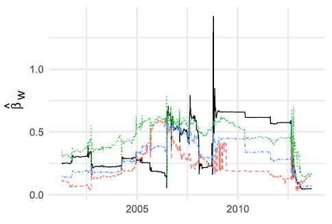
To deal with this non-stationarity, or more generally to deal with parameter drift that is difficult to model explicitly⁴, the standard¹² approach in the litterature is to use a rolling window procedure¹³ for the least squares estimation of the HAR model parameters.

Insanity filter

The HAR volatility forecasting model may on rare occasions generate implausibly large or small forecasts⁴, because no restrictions on the parameters [$\beta$, $\beta_d$, $\beta_w$ and $\beta_m$] are imposed¹¹.

In particular, it has been noted¹⁴ that forecasts are occasionally negative¹¹.

In order to correct this behaviour, Clements and Preve⁴ propose to implement an insanity filter¹⁵ ensuring that any forecast greater than the maximum, or less than the minimum, of [an asset next days’s conditional variance] observed in the estimation period is replaced by the sample average over that period⁴.

Two important remarks on such a filter:

• It seems that the particular choice of insanity filter is not important; what matters is to eliminate unrealistic forecasts¹⁶.
• The presence of an insanity filter is all the more important when an indirect multi-step ahead forecast scheme is used for estimating an asset next $h$-day’s ahead volatility, because an unreasonable [forecast] is most likely to generate another unreasonable forecast¹⁶.

Variance proxies transformations

Clements and Preve⁴ study three different Box-Cox transformations of an asset daily realized variance that can be used in the HAR volatility forecasting model instead of that asset “raw” daily realized variance:

• The logarithmic transformation (log)
• The quartic root transformation (qr)
• The square root transformation (sqr)

It is visible on Figure 2 that these transformations appear useful for reducing skewness, and hence the possible effect of outliers and potential heteroskedasticity in the realized variance series⁴.

Figure 2. S&P 500 index daily realized variance, raw v.s. transformed, 6th April 2001 - 29th August 2013, Source: Clements and Preve.

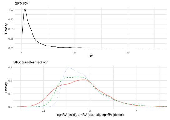
Of particular interest is the logarithmic transformation¹⁷, which in addition to good practical performances and closed form bias-corrected expressions for variance forecasts¹⁸, also guarantees that the generated forecasts are always positive¹⁹.

Non-overlapping daily, weekly and monthly variance proxies

Corsi et al.²⁰ propose a slightly different parametrization of the HAR model compared to Corsi², where:

• $\tilde{\sigma}^2_{T}, \tilde{\sigma}^2_{T-1},…,\tilde{\sigma}^2_{T-21}$ are the asset daily variance estimators over each of the previous 22 days at times $T$, $T-1$, …, $T-21$
• $\tilde{\sigma}^{2,w}_{T} = \frac{1}{4} \sum_{i=2}^5 \tilde{\sigma}^2_{T+1-i}$ is the asset weekly variance estimator at time $T$, non-overlapping with the asset daily variance estimator $\tilde{\sigma}^2_{T}$
• $\tilde{\sigma}^{2,m}_{T} = \frac{1}{17} \sum_{i=6}^{22} \tilde{\sigma}^2_{T+1-i}$ is the asset monthly variance estimator at time $T$, non-overlapping with either the asset daily variance estimator $\tilde{\sigma}^2_{T}$ nor with the asset weekly variance estimator $\tilde{\sigma}^{2,w}_{T}$

Such a re-parametrization does not imply any loss of information compared to the original [HAR model], since it relies only on a different rearrangement of the terms²⁰, but allows an easiest interpretation of the HAR model parameters, c.f. Patton and Sheppard¹¹.

Incidentally, this non-overlapping formulation of the HAR volatility forecasting model has been found to generate better forecasts by practitioners²¹.

Other lag indexes for the variance proxies

The standard lag indexes for the variance proxies in the HAR volatility forecasting model are 1, 5 and 22, each corresponding to a different volatility component in Corsi’s underlying additive cascade model.

As mentioned in Corsi², more components could easily be added to the additive cascade of partial volatilities², which is done for example in Lyocsa et al.⁷.

In that case, denoting $l$ and $h$, respectively, the lowest and highest frequency in the cascade², an asset next days’s conditional variance is modeled as an AR($\frac{l}{h}$) process reparameterized in a parsimonious way by imposing economically meaningful restrictions².

Implementation in Portfolio Optimizer

Portfolio Optimizer implements the HAR volatility forecasting model - augmented with the insanity filter described in Clements and Preve⁴ - through the endpoint /assets/volatility/forecast/har.

This endpoint supports the 4 variance proxies below:

• Squared close-to-close returns
• Demeaned squared close-to-close returns
• The Parkinson range
• The jump-adjusted Parkinson range

This endpoint also supports:

• Transforming the input variance proxies into log variance proxies before estimating the HAR model parameters; the associated variance forecasts are then unbiased thanks to the formulas established in Buccheri and Corsi¹⁸.

• Estimating the HAR model parameters through 3 different least squares procedures:
  • Ordinary least squares
  • Weighted least squares, using the inverse of the variance proxies as weights
  • Robust least squares, using Tukey’s biweight loss function
• Using up to 5 lag indexes for the variance proxies

Example of usage - Volatility forecasting at monthly level for various ETFs

As an example of usage, I propose to enrich the results of the previous blog post, in which monthly forecasts produced by different volatility models are compared - using Mincer-Zarnowitz²² regressions - to the next month’s close-to-close observed volatility for 10 ETFs representative¹⁷ of misc. asset classes:

• U.S. stocks (SPY ETF)
• European stocks (EZU ETF)
• Japanese stocks (EWJ ETF)
• Emerging markets stocks (EEM ETF)
• U.S. REITs (VNQ ETF)
• International REITs (RWX ETF)
• U.S. 7-10 year Treasuries (IEF ETF)
• U.S. 20+ year Treasuries (TLT ETF)
• Commodities (DBC ETF)
• Gold (GLD ETF)

Vanilla HAR volatility forecasting model

Averaged results for all ETFs/regression models over each ETF price history²³ are the following²⁴, when using the vanilla HAR volatility forecasting model:

Volatility model	Variance proxy	$\bar{\alpha}$	$\bar{\beta}$	$\bar{R^2}$
Random walk	Squared close-to-close returns	5.8%	0.66	44%
SMA, optimal $k \in \left[ 1, 5, 10, 15, 20 \right]$ days	Squared close-to-close returns	5.8%	0.68	46%
EWMA, optimal $\lambda$	Squared close-to-close returns	4.7%	0.73	45%
GARCH(1,1)	Squared close-to-close returns	-1.3%	0.98	43%
HAR	Squared close-to-close returns	-0.7%	0.95	46%
Random walk	Parkinson range	5.6%	0.94	44%
SMA, optimal $k \in \left[ 1, 5, 10, 15, 20 \right]$ days	Parkinson range	5.1%	1.00	47%
EWMA, optimal $\lambda$	Parkinson range	4.3%	1.06	48%
GARCH(1,1)	Parkinson range	2.7%	1.18	47%
HAR	Parkinson range	0.1%	1.25	44%
Random walk	Jump-adjusted Parkinson range	4.9%	0.70	45%
SMA, optimal $k \in \left[ 1, 5, 10, 15, 20 \right]$ days	Jump-adjusted Parkinson range	5.1%	0.71	47%
EWMA, optimal $\lambda$	Jump-adjusted Parkinson range	4.0%	0.76	45%
GARCH(1,1)	Jump-adjusted Parkinson range	-1.0%	1.00	45%
HAR	Jump-adjusted Parkinson range	-1.4%	0.99	47%

Alternative HAR volatility forecasting models

Averaged results for all ETFs/regression models over each ETF price history²³ are the following²⁴, when using different variations of the vanilla HAR volatility forecasting model:

Volatility model	Variance proxy	$\bar{\alpha}$	$\bar{\beta}$	$\bar{R^2}$
HAR	Squared close-to-close returns	-0.7%	0.95	46%
HAR (weighted least squares)	Squared close-to-close returns	3.1%	0.71	34%
HAR (robust least squares)	Squared close-to-close returns	-12.3%	2.50	26%
HAR (log)	Squared close-to-close returns	0.5%	0.62	40%
HAR (log, weighted least squares)	Squared close-to-close returns	10%	0.26	13%
HAR (log, robust least squares)	Squared close-to-close returns	0.5%	0.53	40%
HAR	Parkinson range	0.1%	1.25	44%
HAR (weighted least squares)	Parkinson range	0.1%	1.19	44%
HAR (robust least squares)	Parkinson range	-4.2%	2.20	40%
HAR (log)	Parkinson range	1.9%	1.22	50%
HAR (log, weighted least squares)	Parkinson range	-0.6%	1.47	47%
HAR (log, robust least squares)	Parkinson range	2.2%	1.22	50%
HAR	Jump-adjusted Parkinson range	-1.4%	0.99	47%
HAR (weighted least squares)	Jump-adjusted Parkinson range	-4.2%	0.92	46%
HAR (robust least squares)	Jump-adjusted Parkinson range	-6.6%	1.76	41%
HAR (log)	Jump-adjusted Parkinson range	0.9%	0.92	51%
HAR (log, weighted least squares)	Jump-adjusted Parkinson range	-0.8%	1.06	48%
HAR (log, robust least squares)	Jump-adjusted Parkinson range	1.2%	0.92	51%

Comments

From the results of the two previous subsections, it is possible to make the following comments:

• When using squared returns as a variance proxy, the vanilla HAR model is the best volatility forecasting model among all the alternative HAR models as well as among all the models already studied in this series.
• When using the Parkinson range or the jump-adjusted Parkinson range as variance proxies, the log HAR model exhibits the highest r-squared among all the models already studied in this series.
• When using the jump-adjusted Parkinson range as a variance proxy, the log HAR model is the best volatility forecasting model in this series (relatively low bias, highest r-squared).
• When using alternative least square estimators, the forecasts quality generally degrades

Conclusion

The previous section empirically demonstrated that the HAR volatility forecasting model, despite its native relationship with realized variance, is still accurate when used with range-based variance estimators at a long forecasting horizon, in line with Lyocsa et al.⁶

In that context, the (log) HAR model is also the most accurate volatility forecasting model studied so far in this series on volatility forecasting by weighted moving average models!

As usual, feel free to connect with me on LinkedIn or to follow me on Twitter.

–

1. See Boudoukh, J., Richardson, M., & Whitelaw, R.F. (1997). Investigation of a class of volatility estimators, Journal of Derivatives, 4 Spring, 63-71. ↩ ↩²

2. See Fulvio Corsi, A Simple Approximate Long-Memory Model of Realized Volatility, Journal of Financial Econometrics, Volume 7, Issue 2, Spring 2009, Pages 174–196. ↩ ↩² ↩³ ↩⁴ ↩⁵ ↩⁶ ↩⁷ ↩⁸ ↩⁹ ↩¹⁰ ↩¹¹ ↩¹² ↩¹³ ↩¹⁴

3. See Clements, Adam and Preve, Daniel P. A. and Tee, Clarence, Harvesting the HAR-X Volatility Model. ↩ ↩² ↩³ ↩⁴ ↩⁵

4. See Adam Clements, Daniel P.A. Preve, A Practical Guide to harnessing the HAR volatility model, Journal of Banking & Finance, Volume 133, 2021. ↩ ↩² ↩³ ↩⁴ ↩⁵ ↩⁶ ↩⁷ ↩⁸ ↩⁹ ↩¹⁰ ↩¹¹ ↩¹² ↩¹³ ↩¹⁴ ↩¹⁵ ↩¹⁶ ↩¹⁷ ↩¹⁸ ↩¹⁹ ↩²⁰ ↩²¹

5. This additive cascade model is autoregressive in (daily) realized variance and combines realized variance over different horizons (daily, weekly, monthly), hence its name. ↩

6. See Stefan Lyocsa, Peter Molnar, Tomas Vyrost, Stock market volatility forecasting: Do we need high-frequency data?, International Journal of Forecasting, Volume 37, Issue 3, 2021, Pages 1092-1110. ↩ ↩²

7. See Stefan Lyocsa, Tomas Plihal, Tomas Vyrost, FX market volatility modelling: Can we use low-frequency data?, Finance Research Letters, Volume 40, 2021, 101776. ↩ ↩²

8. These three volatility estimators are described in details in a previous blog post. ↩

9. See Brooks, Chris and Persand, Gitanjali (2003) Volatility forecasting for risk management. Journal of Forecasting, 22(1). pp. 1-22. ↩ ↩²

10. Also called iterated scheme. ↩

11. See Andrew J. Patton, Kevin Sheppard; Good Volatility, Bad Volatility: Signed Jumps and The Persistence of Volatility. The Review of Economics and Statistics 2015; 97 (3): 683–697. ↩ ↩² ↩³ ↩⁴

12. Some papers like Buccheri and Corsi¹⁸ describe how to explicitely model the HAR model parameters as time-varying, but in that case, those parameters are not anymore obtained through a simple least squares regression… ↩

13. The length of the rolling window is typically 1000 days, corresponding approximately to 1000 days of trading; more details on the rolling window procedure can be found in Clements et al.³ and a numerical comparison in terms of out-of-sample volatility forecasts between an expanding and a rolling window procedure can be found in Clements and Preve⁴. ↩

14. And I confirm from practical experience. ↩

15. Such a filter has apparently a long history in the forecasting litterature, dating back at least to Swanson and White²⁵ in the context of neural-network models for interest rates forecasting. ↩

16. See Cunha, Ronan, Kock, Anders Bredahl and Pereira, Pedro L. Valls, Forecasting large covariance matrices: comparing autometrics and LASSOVAR. ↩ ↩²

17. Already hinted at in Corsi². ↩ ↩²

18. See Giuseppe Buccheri, Fulvio Corsi, HARK the SHARK: Realized Volatility Modeling with Measurement Errors and Nonlinear Dependencies, Journal of Financial Econometrics, Volume 19, Issue 4, Fall 2021, Pages 614–649. ↩ ↩² ↩³

19. Which helps limiting the need for an insanity filter. ↩

20. See Fulvio Corsi, Nicola Fusari, Davide La Vecchia, Realizing smiles: Options pricing with realized volatility, Journal of Financial Economics, Volume 107, Issue 2, 2013, Pages 284-304. ↩ ↩²

21. See Salt Financial, The Layman’s Guide to Volatility Forecasting: Predicting the Future, One Day at a Time, Research Note. ↩

22. See Mincer, J. and V. Zarnowitz (1969). The evaluation of economic forecasts. In J. Mincer (Ed.), Economic Forecasts and Expectations. ↩

23. The common ending price history of all the ETFs is 31 August 2023, but there is no common starting price history, as all ETFs started trading on different dates. ↩ ↩²

24. For all models, I used an expanding window for the volatility forecast computation. ↩ ↩²

25. See Swanson, N. R. and H. White (1995). A model-selection approach to assessing the information in the term structure using linear models and artificial neural networks. Journal of Business & Economic Statistics 13 (3), 265–275. ↩