Value at Risk: Univariate Estimation Methods

Value-at-Risk (VaR) is one of the most commonly used risk measures in the financial industry¹ in part thanks to its simplicity - because VaR reduces the market risk associated with any portfolio to just one number² - and in part due to regulatory requirements (Basel market risk frameworks³⁴, SEC Rule 18f-4⁵…).

Nevertheless, when it comes to actual computations, the above definition is by no means constructive¹ and accurately estimating VaR is a very challenging statistical problem² for which several methods have been developed.

In this blog post, I will describe some of the most well-known univariate VaR estimation methods, ranging from non-parametric methods based on empirical quantiles to semi-parametric methods involving kernel smoothing or extreme value theory and to parametric methods relying on distributional assumptions.

Value-at-Risk

Definition

The Value-at-Risk of a portfolio of financial instruments corresponds to the maximum potential change in value of [that portfolio] with a given probability over a certain horizon².

More formally, the Value-at-Risk $VaR_{\alpha}$ of a portfolio over a time horizon $T$ (1 day, 10 days, 20 days…) and at a confidence level $\alpha$% $\in ]0,1[$ (95%, 97.5%, 99%…) can be defined⁶ as the opposite⁷ of the $1 - \alpha$ quantile of the portfolio return distribution over the time horizon $T$

\[\text{VaR}_{\alpha} = - \inf_{x} \left\{x \in \mathbb{R}, P(X \leq x) \geq 1 - \alpha \right\}\]

, where $X$ is a random variable representing the portfolio return over the time horizon $T$.

This formula is also equivalent⁸ to

\[\text{VaR}_{\alpha} = - F_X^{-1}(1 - \alpha)\]

, where $F_X^{-1}$ is the inverse cumulative distribution function, also called the quantile function, of the random variable $X$.

Graphically, this definition is illustrated in:

• Figure 1, for a continuous portfolio return distribution at a generic confidence level $\alpha$% and over a generic horizon.

  

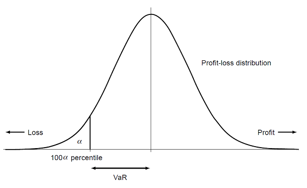
  Figure 1. Graphical illustration of a portfolio VaR as a quantile of its continuous return distribution. Source: Adapted from Yamai and Yoshiba.

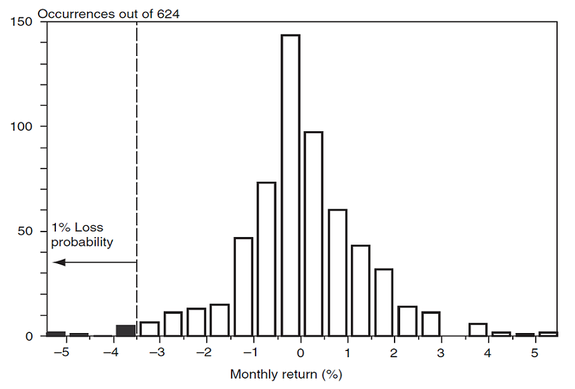
• Figure 2, for a discrete portfolio return distribution at a confidence level $\alpha$ = 99% and over a 1-month horizon, which is commented as follows in Jorion⁹:

  We need to find the loss that will not be exceeded in 99% of cases, or such that 1% of [the 624] observations - that is, 6 out of 624 occurrences - are lower. From Figure [2], this number is about -3.6%, [resulting in a portfolio VaR of 3.6%].

  

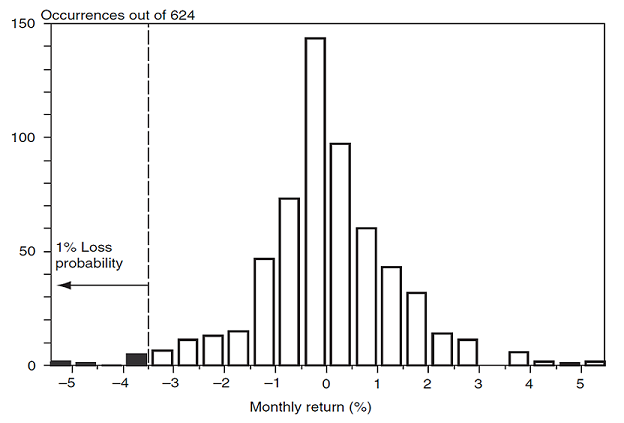
  Figure 2. Graphical illustration of a portfolio VaR as a quantile of its discrete monthly return distribution, $\alpha$ = 99%. Source: Jorion.

Univariate v.s. multivariate Value-at-Risk

A portfolio can be considered as both:

• An asset in itself, with its own return distribution.
• A weighted collection of individual assets, each with their own return distribution.

This raises the question of whether first to aggregate profit and loss data and proceed with a univariate [VaR] model for the aggregate, or to start with disaggregate data¹⁰ and proceed with a multivariate VaR model from the disaggregated data.

In this blog post, I will only discuss univariate¹¹ VaR models - originally suggested by Zangari¹² as simple and effective approach[es] for calculating Value-at-Risk¹² - in which portfolio returns are considered as a univariate time series without reference to the portfolio constituents¹³.

Indeed, since the goal of VaR is to measure the market risk of a portfolio, it seems reasonable to model the portfolio return series directly¹².

Arithmetic returns v.s. logarithmic returns in Value-at-Risk calculations

In VaR calculations, it is usually prefered, for a variety of reasons, to work with logarithmic returns rather than arithmetic (simple, linear) ones¹³, c.f. Ballotta¹³ and Jorion⁹ for more details.

In that case, though, because investors are primarily interested in simple returns¹⁴, the logarithmic VaR $\text{VaR}_{\alpha}^{(l)} $ needs to be converted into an arithmetic VaR $\text{VaR}_{\alpha}^{(a)} $.

Thanks to the definition of VaR as a quantile of the portfolio return distribution and the relationship between arithmetic and logarithmic returns, this is easily be done through the formula

\[\text{VaR}_{\alpha}^{(a)} = 1 - \exp \left( - \text{VaR}_{\alpha}^{(l)} - 1 \right)\]

While not frequently mentioned in the litterature¹⁵, it is important to be aware of this subtlety.

History of Value-at-Risk

Searching for the best means to represent the risk exposure of a financial institution’s trading portfolio in a single number¹⁶ is a quest that folklore attributes the inception of to Dennis Weatherstone at J.P. Morgan [in the late 1980s], who was looking for a way to convey meaningful risk exposure information to the financial institution’s board without the need for significant technical expertise on the part of the board members¹⁶.

It is then Till Guldimann, head of global research at J.P. Morgan at that time, who designed what would come to be known as the J.P. Morgan’s daily VaR report¹⁷ and who thus can be viewed as the creator of the term Value-at-Risk⁹.

The interested reader is referred to Holton¹⁸ for an historical perspective on Value-at-Risk, in which the origins of VaR as a measure of risk are even traced back as far as 1922 to capital requirements the New York Stock Exchange imposed on member firms¹⁸.

Value-at-Risk estimation

When a sample of portfolio returns over a given time horizon $r_1,…,r_n$ is available - like in ex post analysis -, the Value-at-Risk of that portfolio over the same horizon¹⁹ at a confidence level $\alpha \in ]0,1[$ is a textbook example of VaR calculation as the opposite of the $(1 - \alpha)$% quantile of the empirical return distribution $r_1,…,r_n$.

Problem is, the discrete nature of the extreme returns of interest makes it difficult to accurately compute that quantile, as explained in Danielsson and de Vries²⁰:

In the interior, the empirical sampling distribution is very dense, with adjacent observations very close to each other. As a result the sampling distribution is very smooth in the interior and is the mean squared error consistent estimate of the true distribution.

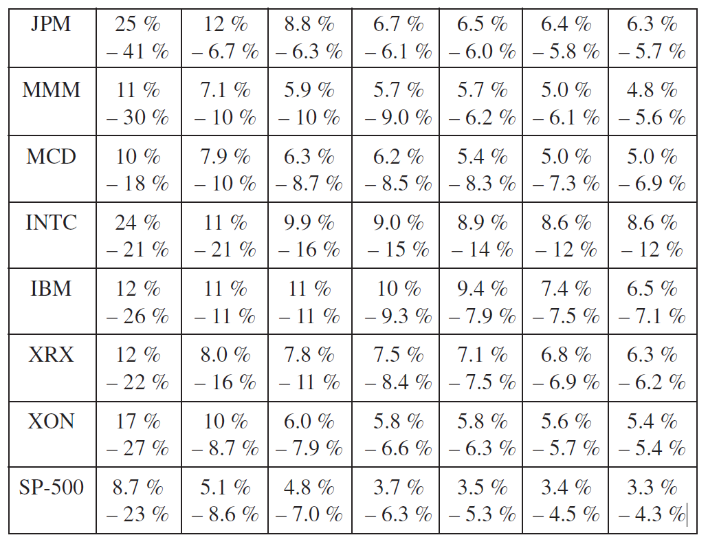
The closer one gets to the extremes, the longer the interval between adjacent returns becomes. This can be seen in [Figure 3] where the 7 largest and smallest returns on the stocks in the sample portfolio and SP-500 Index for 10 years are listed. These extreme observations are typically the most important for VaR analysis, however since these values are clearly discrete, the VaR will also be discrete, and hence be either underpredicted or overpredicted.

Figure 3. Extreme daily returns for select U.S. stocks and S&P 500, 1987-1996. Source: Danielsson and de Vries.

In other words, the quantile corresponding to the estimation of the Value-at-Risk […] rather depends on the realizations of the [portfolio returns] than on their probability distribution¹, so that the Value-at-Risk calculated with a quantile of the empirical distribution will be highly unstable, especially when considering a Value-at-Risk with a high confidence level with only few available data¹.

This is why VaR estimation is a very challenging statistical problem², sharing many similarities with the problem of estimating the frequency and/or severity of extreme events in other domains, like floods frequency estimation²¹ in hydrology.

In order to compute a statistical estimator of a portfolio Value-at-Risk, three main approaches exist:

• Non-parametric approaches, that do not make any specific distributional assumptions on the portfolio return distribution and whose VaR estimators do not depend on any auxiliary parameter.

• Semi-parametric approaches, that do not make any specific distributional assumptions on the portfolio return distribution but whose VaR estimators depend on one or several auxiliary parameters.

• Parametric approaches, that make a specific distributional assumption on the portfolio return distribution and whose VaR estimators depend on one or several auxiliary parameters.

To be noted that non-parametric and semi-parametric approaches might still make distributional assumptions, in particular for convergence proofs - like assuming that returns are independent and identically distributed (i.i.d.) -, but these assumptions are then generic in nature, contrary to parametric approaches which assume a very specific return distribution, like a Gaussian distribution, which is one of the most widely applied parametric probability distribution²² in finance.

Non-parametric and semi-parametric Value-at-Risk estimation

Chen and Yong Tang²³ notes that non-parametric and semi-parametric VaR estimators have the advantages of (i) being free of distributional assumptions […] while being able to capture fat-tail and asymmetry distribution of returns automatically; and (ii) imposing much weaker assumptions on the dynamics of the return process and allowing data “speak for themselves”²³.

Empirical quantile of the portfolio return distribution

A well-known estimator of the $(1 - \alpha)$% quantile of any probability distribution is the empirical $(1 - \alpha)$% quantile of that distribution, which relies on order statistics.

In the context of VaR estimation, the underlying idea is explained in Dowd²⁴:

If we have a sample of $n$ profit and loss (P/L) observations, we can regard each observation as giving an estimate of VaR at an implied probability level. For example, if $n$ = 100, we can take the 5% VaR as the negative of the sixth²⁵ smallest P/L observation, the 1% VaR as the negative of the second-smallest, and so on.

This leads to the empirical portfolio VaR estimator, defined²⁶ as the opposite of the $n (1 - \alpha) + 1$-th highest portfolio return²⁷

\[\text{VaR}_{\alpha} = -r_{\left( n (1 - \alpha) + 1 \right)}\]

, where $r_{(1)} \leq r_{(2)} \leq … \leq r_{(n-1)} \leq r_{(n)}$ are the order statistics of the portfolio returns.

Now, due to the discrete nature of the portfolio return distribution, there is little chance that $n (1 - \alpha) + 1$ is an integer.

In that case, two²⁶ possible choices are:

• Either to define the opposite of the $\lfloor n (1 - \alpha) \rfloor + 1$-th highest portfolio return²⁷ as the empirical portfolio VaR estimator²⁴

  \[\text{VaR}_{\alpha} = - r_{\left( \lfloor n (1 - \alpha) \rfloor + 1 \right)}\]

• Or to define a linear interpolation²⁸ between the opposite of the $\lfloor (n+1) \left( 1 - \alpha \right) \rfloor $-th and $ \lfloor (n+1) \left( 1 - \alpha \right) \rfloor + 1$-th highest portfolio returns²⁷ as the empirical portfolio VaR estimator²⁹³⁰¹³

  \[\text{VaR}_{\alpha} = - \left( 1 - \gamma \right) r_{\left( \lfloor (n+1) \left( 1 - \alpha \right) \rfloor \right)} - \gamma r_{\left( \lfloor (n+1) \left( 1 - \alpha \right) \rfloor + 1 \right)}\]

  , with $\gamma$ $= (n+1) \left( 1 - \alpha \right)$ $- \lfloor (n+1) \left( 1 - \alpha \right) \rfloor$.

An interesting property of the resulting portfolio VaR estimator is that it is consistent in the presence of weak dependence³¹ between portfolio returns, c.f. Chen and Yong Tang²³.

In terms of drawbacks, the two major limitations of the empirical portfolio VaR estimator are that:

• It only takes into account a small part of the information contained in the [portfolio returns] distribution function¹ - that is, at most two returns - which is highly inefficient, especially when the number of portfolio returns is already relatively small.
• It cannot generate any information about the tail of the return distribution beyond the smallest sample observation¹⁶, which might lead to severly underestimate the true risk of the portfolio.

Kernel-smoothed quantile of the portfolio return distribution

Another way to account for the information available in the empirical […] distribution¹ than using the empirical quantile estimator discussed in the previous sub-section is to use the kernel-smoothed quantile estimator introduced in Gourieroux et al.³².

Kernel-smoothing is a methodology belonging to statistics and probability theory that can be thought of as a way of generalizing a histogram constructed with the sample data¹⁶, as illustrated in Figure 4.

Figure 4. Histogram v.s. kernel-smoothed density for the same sample of data. Source: Wikipedia.

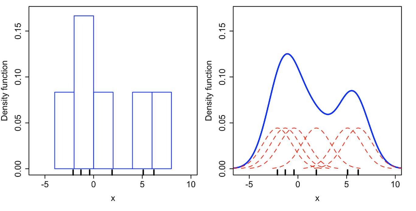
On Figure 4, where a histogram results in a density that is piecewise constant, a kernel[-smoothed} approximation results in a smooth density²³.

Coming back to the estimator of Gourieroux et al.³², it is defined as the $(1 - \alpha)$% quantile of a kernel-smoothed approximation of the portfolio return distribution, which essentially results in a weighted average of the order statistics around [$r_{\left( \lfloor n (1 - \alpha) \rfloor + 1 \right)}$] rather than […] a single order statistic²³ or a linear interpolation between two order statistics.

From a practical perspective, that VaR estimator is computed as follows:

• Select a kernel function $K$, usually²³ taken as a symmetric³³ probability density function.

  The theoretical optimal³⁴ choice for such a kernel function is the Epanechnikov kernel, defined as $ K(u) = \frac{3}{4} \left( 1 - u^2 \right) I_{|u| \leq 1}$.

  However, the litterature suggests that the form of the kernel has little effect on the [accuracy] of the [kernel-smoothed approximation of the return distribution]³², mainly because:

  • The theoretical framework used to establish the optimality of the Epanechnikov kernel relies on large asymptotics, moreover in a debatable way³⁵.
  • The performances³⁶ of other commonly used kernel functions are anyway very close to those of the Epanechnikov kernel³⁷.

  So, in applications, the most common²³³² choice for a kernel function is rather the Gaussian kernel, defined as $ K(u) = \frac{1}{\sqrt{2 \pi }} e^{- \frac{u^2}{2} }$.

  As a side note, using a kernel function to approximate the portfolio return distribution might look like a parametric approach to VaR estimation in disguise, but Butler and Schachter¹⁶ explains why this is not the case:

  Note that use of a normal or Gaussian kernel estimator does not make the ultimate estimation of the VaR parametric.

  As the sample size grows, the net sum of all the smoothed points approaches the true [portfolio return distribution], whatever that may be, irrespective of the method of smoothing the data. This is because the influence of each point becomes arbitrarily small as the sample size grows, so the choice of kernel imposes no restrictions on the results.

• Select a kernel bandwidth parameter $h > 0$ for the kernel function.

  Gourieroux et al.³² describes that parameter as follows:

  The bandwidth parameter controls the range of data points that will be used to estimate the distribution.

  A small bandwidth results in a rough distribution that does not improve appreciably on the original data, while a large bandwidth over-smoothes the density curve and erases the underlying structure.

  This latter point is illustrated in Figure 5 and Figure 6.

  

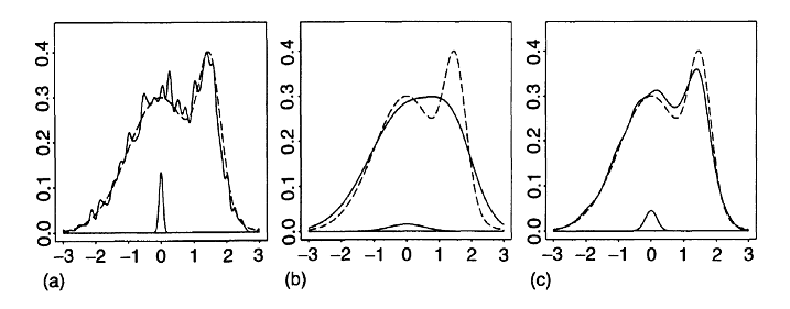
  Figure 5. Influence of the bandwidth parameter on the kernel-smoothed approximation of a normal mixture distribution (dashed) from n = 1000 observations. Source: Adapted from Wand and Jones.

  

  Figure 6. Dynamic influence of the bandwidth parameter on the kernel-smoothed approximation of a normal distribution. Source: KDEpy.

  On Figure 5, it is clearly visible that:

  • a) The estimate of the normal mixture distribution is very rough³⁷.

    This corresponds to a too small bandwidth parameter $h$ that undersmoothes the observations.

  • b) The estimate of the normal mixture distribution smoothes away its bimodality structure.

    This corresponds to a too big bandwidth parameter $h$ that oversmoothes the observations.

  • c) The estimate of the normal mixture distribution is not overly noisy, yet the essential structure of the underlying density has been recovered³⁷.

    This corresponds to an adequate bandwidth parameter $h$.

  On Figure 6, the situation is the same as in Figure 5, except that the bandwidth parameter $h$ is being dynamically increased from 0 to ~20.

  Figure 5 and Figure 6 empirically demonstrate that the choice of the bandwidth is of crucial importance³⁸, although a difficult task, especially when smoothing the tails of underlying distributions with possible data scarcity³⁸.

  The interested reader is refered to Wand and Jones³⁷, Tsybakov³⁵ and Cheng and Sun³⁹ for the description of several methods to choose the optimal bandwidth for a kernel function.

• Compute the kernel-smoothed portfolio VaR estimator as

  \[\text{VaR}_{\alpha} = - \hat{F}^{-1}(1 - \alpha)\]

  , where $ \hat{F}^{-1}(1 - \alpha) $ is the solution of the quantile equation

  \[\hat{F}(x) = \int_{-\infty}^x \hat{f}(u) \, du = 1 - \alpha\]

  with $ \hat{f}(x) = \frac{1}{n h} \sum_{i=1}^n K \left( \frac{x - r_i}{h} \right) $.

  That part is typically done with a numerical algorithm, like the Gauss–Newton algorithm mentioned in Gourieroux et al.³².

Two important positive results on the kernel-smoothed VaR estimator are established in Chen and Yong Tang²³:

• Theoretically, it is consistent in the presence of weak dependence between portfolio returns.

• Empirically, it produces more precise estimates⁴⁰ than those obtained with the empirical VaR estimator - especially when the number of observations is small - which can translate to a large amount in financial terms²³.

  Similar results - in a non-financial context - are reported in Cheng and Sun³⁹:

  It turns out that kernel smoothed quantile estimators, with no matter which bandwidth selection method used, are more efficient than the empirical quantile estimator in most situations.

  And when sample size is relatively small, kernel smoothed estimators are especially more efficient than the empirical quantile estimator.

  In other words, the extra effort of smoothing pays of at the end²³!

The major limitation of the kernel-smoothed VaR estimator, though, is that if the selected kernel function does not reflect the tail features of the true portfolio return distribution, some problems may arise when the quantile to be estimated requires an extrapolation […] far beyond the range of observed data⁴¹.

In the words of Danielsson and de Vries²⁰:

Almost all kernels are estimated with the entire data set, with interior observations dominating the kernel estimation.

While even the most careful kernel estimation will provide good estimates for the interior, there is no reason to believe that the kernel will describe the tails adequately.

Tail bumpiness is a common problem in kernel estimation.

So, while the kernel-smoothed VaR estimator is capable of tail extrapolation - contrary to the empirical VaR estimator - that capability should be used with extreme caution⁴².

A proper portfolio VaR estimator when tail extrapolation is needed thus remains elusive at this stage.

Extrapolated empirical quantile of the portfolio return distribution

In order to solve the problem of tail extrapolation while retaining the simplicity of the empirical quantile estimator, Hutson³⁰ proposes to extend the linearly interpolated quantile function into a tail extrapolation quantile function³⁵ that allows for non-parametric extrapolation beyond the observed data³⁰.

In terms of VaR estimation, Hutson’s work translates into the following extrapolated empirical portfolio VaR estimator:

• For $0 < \left( 1 - \alpha \right) \leq \frac{1}{n+1}$

  \[\text{VaR}_{\alpha} = - r_{(1)} - \left( r_{(2)} - r_{(1)} \right) \log \left( (n+1) \left( 1 - \alpha \right) \right)\]

• For $\left( 1 - \alpha \right) \in ]\frac{1}{n+1} , \frac{n}{n+1}[$, $ \text{VaR}_{\alpha} $ is defined as the standard empirical portfolio VaR estimator

• For $\frac{n}{n+1} < \left( 1 - \alpha \right) < 1$

  \[\text{VaR}_{\alpha} = - r_{(n)} + \left( r_{(n)} - r_{(n-1)} \right) \log \left( (n+1) \alpha \right)\]

Hutson³⁰ establishes the consistency of his quantile estimator for i.i.d. observations and empirically demonstrates using misc. theoretical distributions that it fits well to the ideal sample for all distributions for ideal samples as small as $n = 10$³⁰.

Unfortunately for financial applications, Hutson³⁰ also notes that his quantile estimator appears to be [unable] to completely capture the tail behavior of heavy-tailed⁴³ distributions such as Cauchy³⁰.

This is confirmed by Banfi et al.⁴¹, who finds that Hutson’s method provides competitive results when light-tailed distributions are of interest⁴¹ but generates large biases in the case of heavy-tailed distributions⁴¹.

Extreme value theory-based quantile of the portfolio return distribution

Another possibility to improve [the] tail extrapolation⁴¹ properties of the empirical quantile estimator is to rely on extreme value theory (EVT), which is a domain of statistics concerned with the study of the asymptotical distribution of extreme events, that is to say events which are rare in frequency and huge with respect to the majority of observations⁴⁴.

Indeed, because VaR only deals with extreme quantiles of the distribution⁴⁴, EVT sounds like a natural framework for providing more reliable VaR estimates than the usual ones, given that [it] directly concentrates on the tails of the distribution, thus avoiding a major flaw of [other] approaches whose estimates are somehow biased by the credit they give to the central part of the distribution, thus underestimating extremes and outliers, which are exactly what one is interested in when calculating VaR⁴⁴.

Two preliminary remarks before proceeding:

• One notational

  The EVT litterature⁴⁵ typically focuses on the upper tail of distributions, so that the portfolio returns $r_1,…,r_n$ need to be replaced by their opposites $r^{‘}_1 = -r_1$,…,$r^{‘}_n=-r_n$.

• One important for applying EVT results in finance

  Most existing EVT methods require [i.i.d.] observations, whereas financial time series exhibit obvious serial dependence features such as volatility clustering⁴⁴.

  It turns out that this issue has been addressed in works dealing with weak serial dependence [and] the main message from these studies is that usual EVT methods are still valid⁴⁴.

  For example, the Hill estimator discussed below has originally been derived under the assumptions of i.i.d. observations⁴⁶, but it has also been proved to be usable with weakly dependent observations⁴⁷; the same applies⁴⁸ to the Weissman quantile estimator also discussed below.

  In addition, even though the [EVT] estimators obtained may be less accurate and neglecting this fact could lead to inadequate resolutions in order to cope with the risk of occurrence of extreme events⁴⁴, they are consistent and unbiased in the presence of higher moment dependence¹⁴ and it is even possible to explicitly model extreme dependence using the [notion of] extremal index¹⁴.

With these remarks in mind, EVT offers two main methods¹⁴ to model the upper tail of the portfolio return distribution $r^{‘}_1$,…,$r^{‘}_n$ and compute an EVT-based portfolio VaR estimator:

• A fully parametric method based on the generalized Pareto distribution (GPD)
• A semi-parametric method based on the Hill (or similar) estimator

Generalized Pareto distribution-based method

This method consists in fitting a generalized Pareto distribution to the upper tail of the portfolio return cumulative distribution function (c.d.f.) and computing its $\alpha$% quantile.

This is for example done in the seminal paper of McNeil and Frey⁴⁹, in which such a distribution is fitted to the returns⁵⁰ of different financial instruments.

The theoretical justification for this method lies in the Pickands-Balkema-De Hann’s theorem, which states that EVT holds sufficiently far out in the tails such that we can obtain the distribution not only of the maxima but also of other extremely large observations¹⁴.

In practice, fitting a GPD to the upper tail of the portfolio return distribution is a two-step process:

• First, a threshold $r^{‘}_{(n - k)}, k \geq 1$ beyond which returns should be considered as belonging to the upper tail needs to be selected.

  This threshold corresponds to the location parameter $u \in \mathbb{R}$ of the GPD.

  Unfortunately, the choice of how many of the $k$-largest observations should be considered extreme is not straightforward⁴¹ and is actually a central issue to any application of EVT⁴⁴.

  Indeed, as detailled in de Haan et al.⁵¹:

  Theoretically, the statistical properties of EVT-based estimators are established for $k$ such that $k \to \infty$ and $k/n \to 0$ as $n \to \infty$.

  In applications with a finite sample size, it is necessary to investigate how to choose the number of high observations used in estimation.

  For financial practitioners, two difficulties arise: firstly, there is no straightforward procedure for the selection; secondly, the performance of the EVT estimators is rather sensitive to this choice.

  More specifically, there is a bias–variance tradeoff: with a low level of $k$, the estimation variance is at a high level which may not be acceptable for the application; by increasing $k$, i.e., using progressively more data, the variance is reduced, but at the cost of an increasing bias.

  The literature offers some guidance on how to choose an adequate cut-off between the central part and the upper tail of the return distribution but that choice remains notoriously difficult in general, c.f. Benito et al.⁵² for a review.

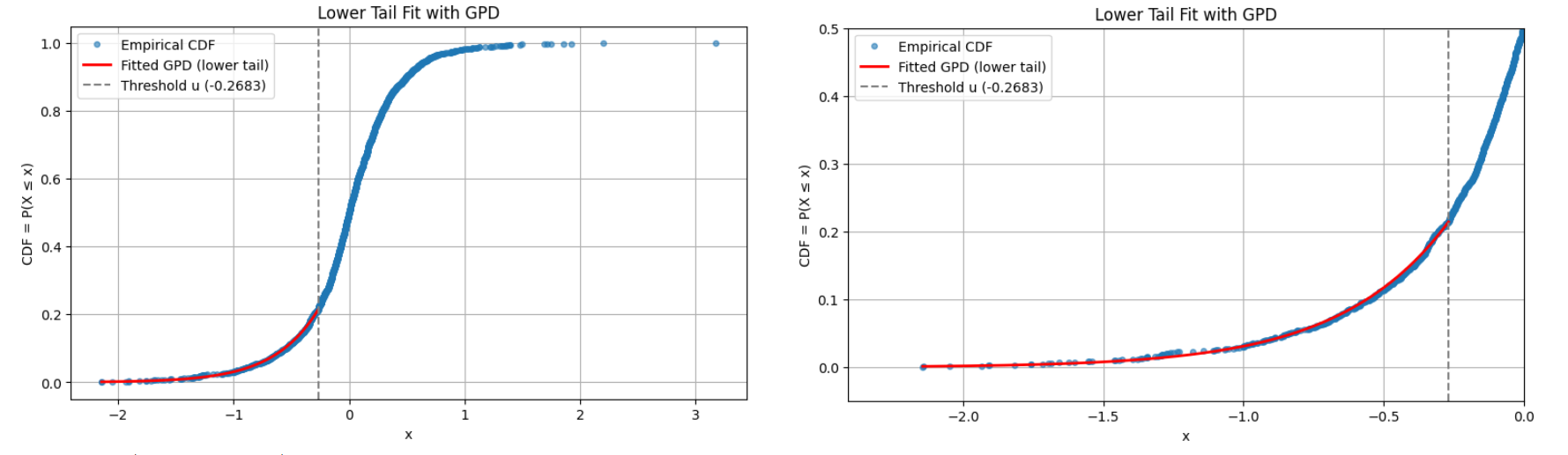
  Fortunately, in the specific context of VaR estimation, there is a large set of thresholds that provide similar GPD quantiles estimators and as a consequence similar market risk measures⁵³ - from about the 80th percentile of observations to the 95th percentile of observations⁵³ - so that the researchers and practitioners should not focus excessively on the threshold choice⁵³.

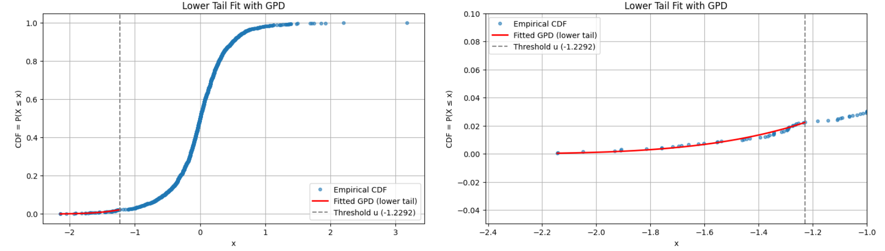
  Figure 7 and Figure 8 illustrate this point with a GPD fitted to the lower tail of daily percentage returns of Deutsche mark/British pound (DEM/GBP) exchange rates from 3rd January 1984 to 31st December 1991⁵⁴, using two different thresholds:

  • Figure 7 - A threshold $u \approx -1.2292$, corresponding to ~2% of the observations.

    

    Figure 7. Lower tail of daily percentage returns of Deutsche mark/British pound (DEM/GBP) exchange rates, GDP fit with threshold u = -1.2292, 3rd January 1984 to 31st December 1991.

  • Figure 8 - A threshold $u \approx -0.2683$, corresponding to ~20% of the observations.

    

    Figure 8. Lower tail of daily percentage returns of Deutsche mark/British pound (DEM/GBP) exchange rates, GDP fit with threshold u = -0.2683, 3rd January 1984 to 31st December 1991.

  From Figure 7 and Figure 8, both thresholds lead to an equally good extreme lower tail GPD fit, which is confirmed numerically by goodness-of-fit measures.

  Consequently, in order to keep the threshold selection step as simple as possible for VaR estimation, the early suggestion of DuMouchel⁵⁵ to use the 90th percentile of observations seems a very good starting point.

• Second, the shape parameter $\xi \in \mathbb{R}$ and the scale parameter $\sigma > 0$ of the GPD need to be estimated.

  This is usually done through likelihood maximization, but other procedures are described in the litterature (method of moments⁵⁶, maximization of goodness-of-fit estimators⁵⁷, etc.).

Once the parameters of the GPD have been determined, the EVT/GPD-based portfolio VaR estimator⁴⁹ is defined as the $\alpha$% quantile of that GPD through the formula

\[\text{VaR}^{\text{GPD}}_{\alpha} = \begin{cases} r^{'}_{(n - k)} + \frac{\hat{\sigma}}{\hat{\xi}} \left( \left( \frac{k}{T ( 1 - \alpha)} \right)^\xi -1 \right) &\text{if } \hat{\xi} \ne 0 \\ r^{'}_{(n - k)} - \hat{\sigma} \ln \frac{T ( 1 - \alpha)}{k} &\text{if } \hat{\xi} = 0 \\ \end{cases}\]

, where:

• $\hat{\xi}$ is an estimator of the shape parameter $\xi$ of the GPD.
• $\hat{\sigma}$ is an estimator of the scale parameter $\sigma$ of the GPD.

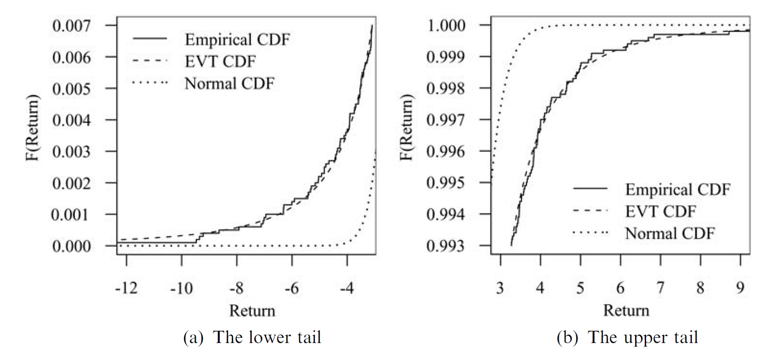
Figure 9, taken from Danielsson ¹⁴, illustrates the near perfect fit that can be obtained when such a method is applied to the upper and lower tails of the daily S&P 500 returns over the period 1970-2009.

Figure 9. Upper and lower tails of daily S&P 500 returns fitted with an EVT-estimated distribution v.s. a normal distribution, 1970-2009. Source: Danielsson.

Hill estimator-based method

Under the assumption that the portfolio return distribution belongs⁵⁸ to the generic family of heavy-tailed distributions, this method consists in deriving an asymptotic estimator of its $\alpha$% quantile.

This is for example done in Danielsson and de Vries⁵⁹ and in Drees⁴⁸.

This method is justified by stylized facts⁶⁰ of asset returns, as explained in Danielsson and de Vries²⁰:

[…] because we know that financial return data are heavy tailed distributed, one can rely on a limit expansion for the tail behavior that is shared by all heavy tailed distributions. The importance of the central limit law for extremes is similar to the importance of the central limit law, i.e. one does not have to choose a particular parametric distribution.

Under that generic assumption, it can be demonstrated⁶¹ that the upper tail of the portfolio returns decays as a power function multiplied by a slowly varying function, that is

\[1 - F(x) = x^{-\gamma} L(x), x > 0\]

, where:

• $F$ is the c.d.f. of the (opposite of the) portfolio returns.
• $\gamma = \frac{1}{\xi} > 0$ is the tail index⁶² of $F$, with $\xi$ the same shape parameter as in the GPD method.
• $L$ is a slowly varying function in a sense defined in Rocco⁴⁴.

From this asymptotic behaviour, the EVT/Weissman-based portfolio VaR estimator is defined as the $\alpha$% Weissman⁶³ quantile estimator of an heavy-tailed distribution through the formula

\[\text{VaR}^{\text{WM}}_{\alpha} = r^{'}_{(n - k)} \left( \frac{k}{n \left( 1 - \alpha \right) } \right)^{\frac{1}{\hat{\gamma}}}\]

, where⁶⁴:

• $\hat{\gamma}$ is an estimator of the tail index $\gamma$.

  The most frequently employed estimator of the tail index is by far the Hill estimator⁴⁴ introduced in Hill⁴⁶ and defined conditionally on $k$ as

  \[\hat{\gamma} = \frac{1}{k} \sum_{i=1}^k \ln \frac{r^{'}_{(n - i + 1)}}{r^{'}_{(n - k)}}\]

  The interested reader is referred to Fedotenkov⁶⁵, in which more than one hundred tail index estimators proposed in the literature are reviewed.

• $k$ is the number of observations $r^{‘}_{(n - k + 1)}$, …, $r^{‘}_{(n)}$ that should be considered extreme.

  Here, and contrary to the GPD method, the threshold index $k$ has a huge influence on the Weissman quantile estimator and thus on the EVT/Weissman-based VaR estimator.

  As an illustration, Figure 10 depicts the daily VaR of the Dow Jones Industrial Average index at a confidence level $\alpha = 99.9$%⁶⁶ as a function of $k$, when estimated by the EVT/Weissman-based VaR estimator.

  

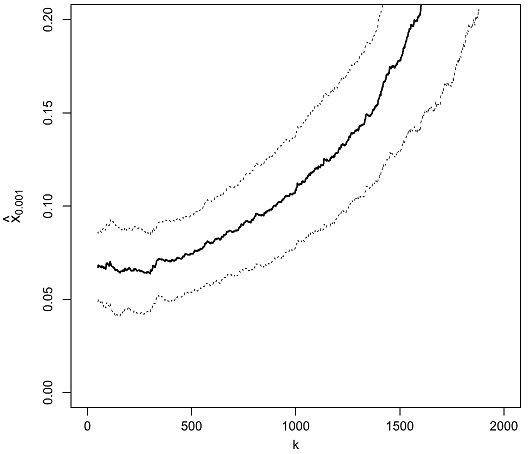
  Figure 10. Impact of the threshold index k between the central part and the upper tail of the Dow Jones Industrial Average daily return distribution, Weissman quantile estimator of VaR 99.9%, 1980-2010. Source: de Haan et al.

  On Figure 10, three distinct ranges of values for the index $k$ are visible:

  • An initial range of values for $k \in [1, 150]$ that results in a bumpy VaR estimate, although on this specific figure the bumpyness is not that pronounced.

    This is the “high variance” region of the estimator.

  • A second range of values for $k \in [150, 300]$ that results in a flat-ish VaR estimate.

    This is the “optimal bias-variance” region of the estimator, in which the exact value of $k$ is not important.

    Obtaining an estimate of $k$ belonging to that region is the ultimate goal.

  • A third range of values for $k \geq 300$ that results in a diverging VaR estimate.

    This is the “high bias” region of the estimator.

  Hopefully, this problem can be solved by using a bias-corrected Weissman quantile estimator.

  For example, Figure 11 depicts the daily VaR of the Dow Jones Industrial Average index at a confidence level $\alpha = 99.9$% as a function of $k$, when estimated by the EVT/unbiased Weissman-based VaR estimator introduced in de Haan et al.⁵¹.

  

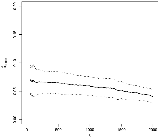
  Figure 11. Impact of the threshold index k between the central part and the upper tail of the Dow Jones Industrial Average daily return distribution, unbiased Weissman quantile estimator of VaR 99.9%, 1980-2010. Source: de Haan et al.

  Comparing Figure 11 to Figure 10, the improvement in stability of the quantile estimator is striking.

One important limitation of this method compared to the GPD-based method is that depending on the exact financial data used (financial instrument, time period, returns frequency…), the stylized heavy tailedness nature of return distributions might be violated, with return distributions being thin-tailed or short-tailed⁶⁷ instead of heavy-tailed, c.f. Longin and Solnik⁶⁷ and Drees⁴⁸.

Indicentally, the two lower tail GPD fits depicted in Figure 7 and Figure 8 both correspond to a short-tailed distribution since $\hat{\xi} \approx -0.2304$ on Figure 7 and $\hat{\xi} \approx -0.021$ on Figure 8.

Practical performances

In terms of practical performances, Danielsson¹⁴ highlights that EVT-based VaR estimation delivers good probability–quantile estimates where EVT holds¹⁴, but that there are no rules that tell us when [EVT] becomes inaccurate¹⁴.

Indeed, it depends on the underlying distribution of the data. In some cases, it may be accurate up to 1% or even 5%, while in other cases it is not reliable even up to 0.1%¹⁴.

In addition, the accuracy of EVT also depends on the selected threshold.

This is illustrated in Figure 12, which is identical to Figure 7 except that the GPD fit has been graphically extended to the right of the threshold $u \approx -1.2292$.

Figure 12. Lower tail of daily percentage returns of Deutsche mark/British pound (DEM/GBP) exchange rates, GDP fit with threshold u = -1.2292 extended, 3rd January 1984 to 31st December 1991.

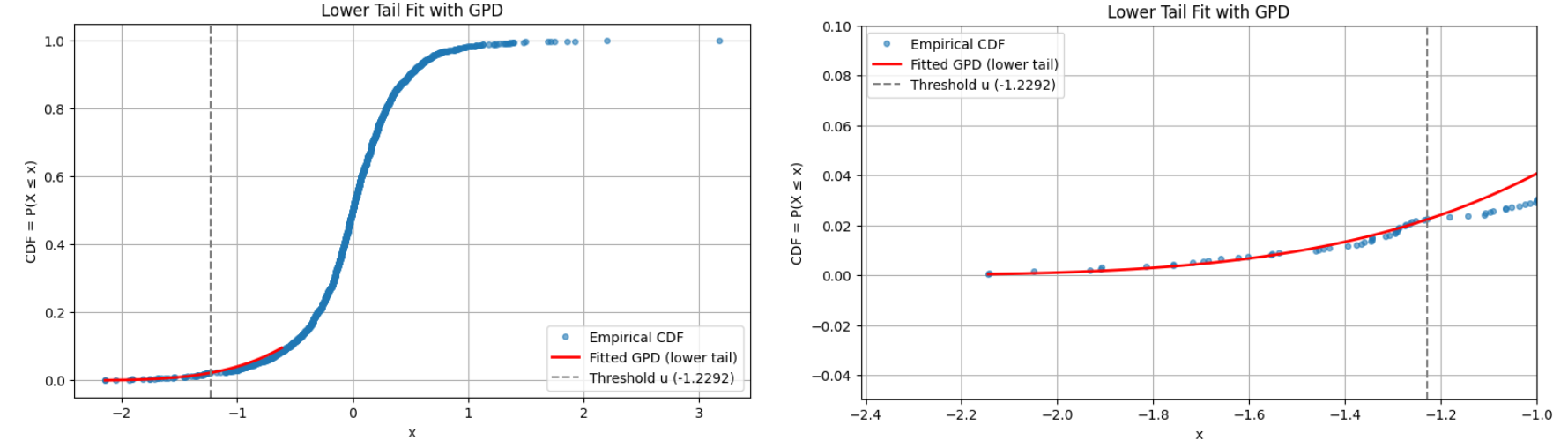
From Figure 7 and Figure 8, both GPT fits seem usable below $u \approx -1.2292$.

But while the GPD fit of Figure 8 is valid up to $u \approx -0.2683$, Figure 12 makes it clear that the GPD fit of Figure 7 is completely off above $u \approx -1.2292$.

Other estimators

It is out of scope of this blog post to list all non-parametric and semi-parametric portfolio VaR estimators discussed in the litterature, but I would like to finish this section by mentionning estimators based on smoothing splines.

An example of such an estimator is described in Shaker-Akhtekhane and Poorabbas⁶⁸, in which it is empirically demonstrated to outperform common historical, parametric, and kernel-based methods⁶⁸ when applied to the S&P500 index at VaR confidence levels of $\alpha = 95$% and $\alpha = 99$%.

Misc. points of attention for such estimators:

• Monotonicity constraints need to be imposed on smoothing splines in order to properly approximate the c.d.f. of the portfolio returns, as highlighted in Wood⁶⁹.

  These are not mentioned in Shaker-Akhtekhane and Poorabbas⁶⁸, but are required in practice.

• Similar to kernel-smoothing, a smoothing parameter needs to be selected.

  The same kind of problems arise, with solutions that are very close in spirit like generalized cross-validation, c.f. Wood⁶⁹.

• Again similar to kernel-smoothing, special care must be taken when extrapolating beyond the range of observed values.

  In particular, the estimator described in Shaker-Akhtekhane and Poorabbas⁶⁸ cannot extrapolate beyond the smallest and the highest portfolio returns due to the splines constraints associated with these two points.

Parametric Value-at-Risk estimation

Contrary to the non-parametric and semi-parametric approaches, parametric - also called analytical - approaches make the assumption⁷⁰ that the whole portfolio return distribution can be described by a parametric distribution $F_{\theta}$ whose parameters $\theta$ need to be estimated from observations.

The $(1 - \alpha)$% quantile of the portfolio return distribution is then simply obtained by inverting that parametric distribution, which leads to the definition of the parametric portfolio VaR estimator as

\[\text{VaR}_{\alpha} = - F_{\theta}^{-1} (1 - \alpha)\]

Parametric approaches thus replace the problem of accurately computing the quantile of an empirical distribution of observations by the problem of choosing a parametric distribution that best fits these observations.

A couple of examples:

• If the portfolio returns are assumed to be distributed according to a Gaussian distribution, the associated portfolio VaR is called Gaussian Value-at-Risk (GVaR) and is computed through the formula⁷¹

  \[\text{GVaR}_{\alpha} (X) = - \mu - \sigma z_{1 - \alpha}\]

  , where:

  • The location parameter $\mu$ and the scale parameter $\sigma$ are usually⁷² estimated by their sample counterparts.
  • $z_{1 - \alpha}$ is the $1 - \alpha$ quantile of the standard normal distribution.

  This is the assumption made in the RiskMetrics model⁷³.

• If the portfolio returns are assumed to be distributed according to an heavy-tailed distribution, several distributions can be used:

  • A Cornish-Fisher distribution, whose associated portfolio VaR is known as Modified Value-at-Risk
  • A Gaussian mixture distribution

  • …

    Here, as a side note, even though it is known that financial time series usually exhibit skewed and fat-tailed distributions⁶⁰, there is no complete agreement on what distribution could fit them best⁴⁴, so that finding the best distribution to use is as much art as science…

Parametric VaR estimation approaches might be very successful, especially with long risk horizons (months, years…) and/or with not too extreme confidence levels (90%, 95%…).

Nevertheless, they might also not be able to provide an adequate description of the whole range of data, resulting in a good fit of the body but a non accurate description of the tails⁴¹, leading to biases in VaR estimates.

Implementation in Portfolio Optimizer

Portfolio Optimizer supports different portfolio Value-at-Risk estimation methods, c.f. the documentation:

• Empirical portfolio VaR estimation
• Extrapolated empirical portfolio VaR estimation

• Kernel-smoothed empirical portfolio VaR estimation

  For that estimation method, the kernel bandwidth parameter $h$ is automatically computed using a proprietary variation of the improved Sheather and Jones rule described in Botev et al.⁷⁴

• EVT-based portfolio VaR estimation (both GPD-based and Hill estimator-based)

  For these estimation methods:

  • The number of extreme observations $k$ is automatically computed using a proprietary variation of the goodness-of-fit procedure described in El-Aroui and Diebolt⁷⁵.
  • The estimated GPD parameters are unbiased through the formulas described in Giles et al.⁷⁶.
  • The estimated Hill and Weissman estimators are unbiased through the formulas described in de Haan et al.⁵¹ and corrected in Chavez-Demoulin and Guillou⁷⁷.

• Parametric portfolio VaR estimation

  The supported parametric distributions are:

  • The Gaussian distribution
  • The Gaussian mixture distribution
  • The Cornish-Fisher distribution

Conclusion

This blog post described some of the most well-known methods for univariate Value-at-Risk estimation.

Thanks to these, it is possible to analyze the past behaviour of a financial portfolio, but their real interest lies in univariate Value-at-Risk forecasting, which will be the subject of the next blog post in this series.

Stay tuned!

Meanwhile, feel free to connect with me on LinkedIn or to follow me on Twitter.

–

1. See Gueant, O., Computing the Value at Risk of a Portfolio: Academic literature and Practionners’ response, EMMA, Working Paper. ↩ ↩² ↩³ ↩⁴ ↩⁵ ↩⁶

2. See Manganelli, Simone and Engle, Robert F., Value at Risk Models in Finance (August 2001). ECB Working Paper No. 75. ↩ ↩² ↩³ ↩⁴

3. Basel II requires⁷⁸ to calculate market risk capital requirements using VaR at a 99% confidence level over a 10-day horizon. ↩

4. Basel III requires⁷⁹ internal backtesting procedures based on VaR and Stress VaR (VaR applied to a market stress period). ↩

5. The SEC Rule 18f-4 requires companies to calculate daily VaR at a 99% confidence level over a 20-day horizon and using at least 3 years of historical data; it also requires companies to backtest their VaR models daily over a 1-day horizon. ↩

6. See Stoyan V. Stoyanov, Svetlozar T. Rachev, Frank J. Fabozzi, Sensitivity of portfolio VaR and CVaR to portfolio return characteristics, Working paper. ↩

7. C.f. Dowd²⁴, the VaR is the negative of the relevant P/L observation because P/L is positive for profitable outcomes and negative for losses, and the VaR is the maximum likely loss (rather than profit) at the specified probability²⁴, so that VaR is a positive percentage; to be noted, though, that VaR can be negative when no loss is incurred within the confidence level, in which case it is meaningless; c.f. Daníelsson¹⁴. ↩

8. This is the case when the portfolio return cumulative distribution function is strictly increasing and continuous; otherwise, a similar formula is still valid, with $F_X^{-1}$ the generalized inverse distribution function of $X$, but these subtleties - important in mathematical proofs and in numerical implementations - are out of scope of this blog post. ↩

9. See Jorion, P. (2007). Value at risk: The new benchmark for managing financial risk. New York, NY: McGraw-Hill. ↩ ↩² ↩³

10. See Keith Kuester, Stefan Mittnik, Marc S. Paolella, Value-at-Risk Prediction: A Comparison of Alternative Strategies, Journal of Financial Econometrics, Volume 4, Issue 1, Winter 2006, Pages 53–89. ↩

11. Also called top-down VaR models¹³ or portfolio aggregation-based models. ↩

12. See Zangari, Peter, 1997, Streamlining the market risk measurement process, RiskMetrics Monitor, 1, 29–35. ↩ ↩² ↩³

13. See Ballotta, L. ORCID: 0000-0002-2059-6281 and Fusai, G. ORCID: 0000-0001-9215-2586 (2017). A Gentle Introduction to Value at Risk. ↩ ↩² ↩³ ↩⁴ ↩⁵

14. See Jon Danielsson, Financial Risk Forecasting: The Theory and Practice of Forecasting Market Risk, with Implementation in R and Matlab, Wiley 2011. ↩ ↩² ↩³ ↩⁴ ↩⁵ ↩⁶ ↩⁷ ↩⁸ ↩⁹ ↩¹⁰ ↩¹¹

15. Danielsson¹⁴ comes to my mind. ↩

16. See J. S. Butler & Barry Schachter, 1996. Improving Value-At-Risk Estimates By Combining Kernel Estimation With Historical Simulation, Finance 9605001, University Library of Munich, Germany. ↩ ↩² ↩³ ↩⁴ ↩⁵

17. That report was required by 4.15pm and originally became known as the 4.15 report. ↩

18. See Glyn A. Holton, (2002), History of Value-at-Risk: 1922-1998, Method and Hist of Econ Thought, University Library of Munich, Germany. ↩ ↩²

19. The two horizons might be different, but this is out of scope of this blog post. ↩

20. See Danielsson, Jon, and Casper G. De Vries. Value-at-Risk and Extreme Returns. Annales d’Économie et de Statistique, no. 60, 2000, pp. 239–70. ↩ ↩² ↩³

21. See Lall, U., Y. Moon, and K. Bosworth (1993), Kernel flood frequency estimators: Bandwidth selection and kernel choice, Water Resour. Res.,29(4), 1003–1015. ↩

22. See RiskMetrics. Technical Document, J.P.Morgan/Reuters, New York, 1996. Fourth Edition. ↩

23. See Song Xi Chen, Cheng Yong Tang, Nonparametric Inference of Value-at-Risk for Dependent Financial Returns, Journal of Financial Econometrics, Volume 3, Issue 2, Spring 2005, Pages 227–255. ↩ ↩² ↩³ ↩⁴ ↩⁵ ↩⁶ ↩⁷ ↩⁸ ↩⁹ ↩¹⁰

24. See Kevin Dowd, Estimating VaR with Order Statistics, The Journal of Derivatives Spring 2001, 8 (3) 23-30 ↩ ↩² ↩³ ↩⁴

25. To be noted that Dowd²⁴ proposes to take the sixth observation as [the] 5% VaR because we want 5% of the probability mass to lie to the left of [the] VaR²⁴, but other auhors propose to use the fifth observation instead¹³²⁹. ↩

26. Many other choices - at least 9 - are possible though, c.f. Hyndman and Fan⁸⁰; ultimately, what is needed is an estimator of the $(1 - \alpha)$% quantile of the empirical portfolio return distribution. ↩ ↩²

27. For $ 1 - \alpha \in ]\frac{1}{n+1} , \frac{n}{n+1}[$, that is, no extrapolation is possible. ↩ ↩² ↩³

28. Such a linearly interpolated quantile estimator has been known since at least Parzen⁸¹. ↩

29. See Peter Hall and Andrew Rieck. (2001). Improving Coverage Accuracy of Nonparametric Prediction Intervals. Journal of the Royal Statistical Society. Series B (Statistical Methodology), 63(4), 717–725. ↩ ↩²

30. See Hutson, A.D. A Semi-Parametric Quantile Function Estimator for Use in Bootstrap Estimation Procedures. Statistics and Computing 12, 331–338 (2002). ↩ ↩² ↩³ ↩⁴ ↩⁵ ↩⁶ ↩⁷

31. To be noted that weak dependence is a kind of misnomer, because this type of dependence actually covers a very broad range of time series models! ↩

32. See Gourieroux, C., Scaillet, O. and Laurent, J.P. (2000). Sensitivity analysis of Values at Risk. Journal of Empirical Finance, 7, 225-245. ↩ ↩² ↩³ ↩⁴ ↩⁵ ↩⁶

33. Asymmetric kernel functions also exist, c.f. for example Abadir and Lawford⁸². ↩

34. In a mean squared-error sense. ↩

35. See Alexandre B. Tsybakov. 2008. Introduction to Nonparametric Estimation (1st. ed.). Springer Publishing Company, Incorporated. ↩ ↩² ↩³

36. The performance of a kernel estimator $K$ is defined in terms of the ratio of sample sizes necessary to obtain the same minimum asymptotic mean integrated squared error (for a given [function $f$ that is being kernel-smoothed] when using $K$ as when using [the Epanechnikov kernel]³⁷. ↩

37. See Wand, M.P., & Jones, M.C. (1994). Kernel Smoothing (1st ed.). Chapman and Hall/CRC. ↩ ↩² ↩³ ↩⁴ ↩⁵

38. See Keming Yu & Abdallah K. Ally & Shanchao Yang & David J. Hand, Kernel quantile based estimation of expected shortfall, Journal of Risk, Journal of Risk. ↩ ↩²

39. See Cheng, M.-Y. and S. Sun (2006). Bandwidth selection for kernel quantile estimation. Journal of the Chinese Statistical Association 44 (3), 271–295. ↩ ↩²

40. Yet, Chen and Yong Tang²³ notes that the reduction in RMSE is not very large for large samples²³, confirming the theoretical results that the reduction is of second order only²³. ↩

41. See Banfi, F., Cazzaniga, G. & De Michele, C. Nonparametric extrapolation of extreme quantiles: a comparison study. Stoch Environ Res Risk Assess 36, 1579–1596 (2022). ↩ ↩² ↩³ ↩⁴ ↩⁵ ↩⁶ ↩⁷

42. Potential solutions to this problem might be to use 1) a data-driven mixture of a Gaussian and a Cauchy kernel as proposed in Banfi et al.⁴¹ or 2) a preliminary transformation of the data with a Champernowne distribution as proposed in Buch-Kromann et al.⁸³. ↩

43. The family of heavy-tailed distributions encompasses all the fat-tailed distributions enocuntered in finance like the Student-t distribution and more. ↩

44. See Rocco, Marco, Extreme Value Theory for Finance: A Survey (February 3, 2012). Bank of Italy Occasional Paper No. 99. ↩ ↩² ↩³ ↩⁴ ↩⁵ ↩⁶ ↩⁷ ↩⁸ ↩⁹ ↩¹⁰

45. See Danielsson, J., de Vries, C., 1997. Tail index and quantile estimation with very high frequency data. Journal of Empirical Finance 4, 241–257. ↩

46. See Hill, B.M. (1975) A Simple General Approach to Inference About the Tail of a Distribution. Annals of Statistics, 3, 1163-1174. ↩ ↩²

47. See B. Karima and B. Youcef, Asymptotic Normality of Hill’s Estimator under Weak Dependence, Statistical Methodologies. IntechOpen, Feb. 26, 2020. ↩

48. See Drees, Holger. Extreme Quantile Estimation for Dependent Data, with Applications to Finance. Bernoulli, vol. 9, no. 4, 2003, pp. 617–57. ↩ ↩² ↩³

49. See Alexander J. McNeil, Rudiger Frey, Estimation of tail-related risk measures for heteroscedastic financial time series: an extreme value approach, Journal of Empirical Finance, Volume 7, Issues 3–4, 2000, Pages 271-300. ↩ ↩²

50. More precisely, to the standardized residuals of an AR(1)-GARCH(1,1) model of these asset returns; the rationale is that excesses over threshold should be more justified with AR(1)-GARCH(1,1) standardized residuals than with raw asset returns. ↩

51. See de Haan, L., Mercadier, C. & Zhou, C. Adapting extreme value statistics to financial time series: dealing with bias and serial dependence. Finance Stoch 20, 321–354 (2016). ↩ ↩² ↩³

52. See Benito S, Lopez-Martín C, Navarro MA. Assessing the importance of the choice threshold in quantifying market risk under the POT approach (EVT). Risk Manag. 2023;25(1). ↩

53. See Benito, S., Lopez-Martín, C. & Navarro, M.A. Assessing the importance of the choice threshold in quantifying market risk under the POT approach (EVT). Risk Manag 25, 6 (2023). ↩ ↩² ↩³

54. See Bollerslev, T., and Ghysels, E. (1996). Periodic Autoregressive Conditional Heteroskedasticity. Journal of Business & Economic Statistics, 14, 139–151. ↩

55. See William H. DuMouchel. “Estimating the Stable Index α in Order to Measure Tail Thickness: A Critique.” Ann. Statist. 11 (4) 1019 - 1031, December, 1983. ↩

56. See J. R. M. Hosking and J. R. Wallis, Parameter and Quantile Estimation for the Generalized Pareto Distribution, Technometrics, Vol. 29, No. 3 (Aug., 1987), pp. 339-349. ↩

57. See Alberto Luceno, Fitting the generalized Pareto distribution to data using maximum goodness-of-fit estimators, Computational Statistics & Data Analysis, Volume 51, Issue 2, 2006, Pages 904-917. ↩

58. In EVT terms, the true portfolio return distribution is assumed to be in the Fréchet domain of attraction. ↩

59. See Danielsson J., de Vries C. G. (1997). Beyond the Sample: Extreme Quantile and Probability Estimation, Mimeo, Tinbergen Institute Rotterdam. ↩

60. See R. Cont (2001) Empirical properties of asset returns: stylized facts and statistical issues, Quantitative Finance, 1:2, 223-236. ↩ ↩²

61. The cumulative distribution function of the portfolio returns is in the maximum domain of attraction of a Fréchet-type extreme value distribution if and only if $1 - F$ has that form, c.f. Rocco⁴⁴. ↩

62. The tail index is also known as the extreme value index. ↩

63. See Weissman, I.: Estimation of parameters and large quantiles based on the k largest observations. J. Am. Stat. Assoc. 73, 812–815 (1978). ↩

64. The formula for the EVT/Weissman-based portfolio VaR estimator is the one in Nieto and Ruiz⁸⁴ and is slightly different from the one in Danielsson and de Vries⁵⁹, c.f. Danielsson¹⁴ in which a general threshold $u$ is used instead of $r^’_{(\hat{k})}$ or $r^’_{(\hat{k}+1)}$. ↩

65. See Fedotenkov, I. (2020). A Review of More than One Hundred Pareto-Tail Index Estimators. Statistica, 80(3), 245–299. ↩

66. As required under Basel III framework⁸⁵. ↩

67. See Longin, F.M., and B. Solnik (1997). Correlation structure of international equity markets during extremely volatile periods. Working Paper 97-039, ESSEC, Cergy-Pontoise, France. ↩ ↩²

68. See Saeed Shaker-Akhtekhane & Solmaz Poorabbas, 2023. Value-at-Risk Estimation Using an Interpolated Distribution of Financial Returns Series, Journal of Applied Finance & Banking, SCIENPRESS Ltd, vol. 13(1), pages 1-6. ↩ ↩² ↩³ ↩⁴

69. See Wood, S. N., Monotonic Smoothing Splines Fitted by Cross Validation, 1994, SIAM Journal on Scientific Computing, 1126-1133, 15, 5. ↩ ↩²

70. In addition, with multivariate VaR models, parametric methods also needs to us[e] approximations of the pricing formulas of each [non simple] asset in the portfolio¹, leading to methods like Delta-Normal or Delta-Gamma-(Theta-)Normal based on Taylor expansions of the assets pricing formulas, c.f. Gueant¹. ↩

71. See Boudt, Kris and Peterson, Brian G. and Croux, Christophe, Estimation and Decomposition of Downside Risk for Portfolios with Non-Normal Returns (October 31, 2007). Journal of Risk, Vol. 11, No. 2, pp. 79-103, 2008. ↩

72. See Martin, R. Douglas and Arora, Rohit, Inefficiency of Modified VaR and ES. ↩

73. Gueant¹ notes that the RiskMetrics model for the distribution of the evolution of the risk factors is based on the assumption that log-returns of prices (or variations in the case of interest rates) are independent across time and normally distributed, when appropriately scaled by an appropriate measure of volatility¹. ↩

74. See Z. I. Botev. J. F. Grotowski. D. P. Kroese. “Kernel density estimation via diffusion.” Ann. Statist. 38 (5) 2916 - 2957, October 2010. ↩

75. See Mhamed-Ali El-Aroui, Jean Diebolt, On the use of the peaks over thresholds method for estimating out-of-sample quantiles, Computational Statistics & Data Analysis, Volume 39, Issue 4, 2002, Pages 453-475. ↩

76. See David E. Giles, Hui Feng & Ryan T. Godwin (2016) Bias-corrected maximum likelihood estimation of the parameters of the generalized Pareto distribution, Communications in Statistics - Theory and Methods, 45:8, 2465-2483. ↩

77. See Valerie Chavez-Demoulin, Armelle Guillou, Extreme quantile estimation for beta-mixing time series and applications, Insurance: Mathematics and Economics, Volume 83, 2018, Pages 59-74. ↩

78. See Basel Committee on Banking Supervision. Revisions to the Basel II market risk framework (Updated as of 31 December 2010). 2011. ↩

79. See Basel Committee on Banking Supervision. Fundamental review of the trading book.. ↩

80. See Hyndman, R. J., & Fan, Y. (1996). Sample Quantiles in Statistical Packages. The American Statistician, 50(4), 361–365. ↩

81. See Parzen E (1979), Nonparametric statistical data modeling, J Am Stat Assoc 74(365):105–121. ↩

82. See Karim M Abadir, Steve Lawford, Optimal asymmetric kernels, Economics Letters, Volume 83, Issue 1, 2004, Pages 61-68. ↩

83. See Buch-Kromann, Tine and Nielsen, Jens Perch and Guillen, Montserrat and Bolancé, Catalina, Kernel Density Estimation for Heavy-Tailed Distributions Using the Champernowne Transformation (January 2005). ↩

84. See Maria Rosa Nieto, Esther Ruiz, Frontiers in VaR forecasting and backtesting, International Journal of Forecasting, Volume 32, Issue 2, 2016, Pages 475-501. ↩

85. Basel III requires⁷⁹ that the VaR measures for risks on both trading and banking books must be calculated at a 99.9% confidence level. ↩