Correlation Matrices Denoising: Results from Random Matrix Theory

The estimation of empirical correlation matrices in finance is known to be affected by noise, in the form of measurement error, due in part to the short length of the time series of asset returns typically used in their computation¹.

Worse, large empirical correlation matrices have been shown to be so noisy that, except for their largest eigenvalues and their associated eigenvectors, they can essentially be considered as random.

For example, Laloux et al.² reports that around 94% of the spectrum of an empirical correlation matrix estimated from the returns of the S&P 500 constituents is indistinguishable from the spectrum of a random correlation matrix!

So, before using an empirical correlation matrix, it is usually advised to denoise it.

In this post, I will present the denoising method proposed by Laloux et al.², based on results from random matrix theory (RMT), and I will illustrate its behaviour in two universes of assets.

Notes:

• An excellent introduction to random matrix theory and some of its applications in finance is the book A First Course in Random Matrix Theory¹ from Marc Potters and Jean-Philippe Bouchaud.

Mathematical preliminaries

In the context of this post, the most important result from random matrix theory is the Marchenko-Pastur theorem, which describes the eigenvalue distribution of large random covariance matrices.

The Marchenko-Pastur theorem

Below is a simple version of the Marchenko-Pastur theorem, in the case of i.i.d. Gaussian observations¹.

Let be:

• $X \in \mathcal{M}(\mathbb{R}^{n \times T})$ an observation matrix made of i.i.d. Gaussian entries with mean 0 and variance $\sigma^2$³
• $\Sigma \in \mathcal{M}(\mathbb{R}^{n \times n})$ the empirical covariance matrix associated to $X$, defined by $\Sigma = \frac{1}{T} X X^t$

Then, given $N \to +\infty$, $T \to +\infty$ and $0 < q = \frac{n}{T} \leq 1$, the density of eigenvalues of the matrix $\Sigma$ converges to the Marchenko-Pastur density defined by

\[\rho_{MP}(\lambda) = \begin{cases} \frac{\sqrt{\left(\lambda_{+} - \lambda\right)\left(\lambda - \lambda_{-}\right)}}{2 \pi q \sigma^2}, \textrm{if } \lambda \in [\lambda_{+}, \lambda_{-}] \newline 0, \textrm{if } \lambda \notin [\lambda_{+}, \lambda_{-}] \end{cases}\]

, with $\lambda_{-}$ the lower edge of the spectrum defined by

\[\lambda_{-} = \sigma^2 \left(1 - \sqrt q \right)^2\]

and $\lambda_{+}$ the upper edge of the spectrum defined by

\[\lambda_{+} = \sigma^2 \left(1 + \sqrt q \right)^2\]

To be noted that, under proper technical assumptions, the Marchenko-Pastur theorem remains valid for observations drawn from more general distributions, like fat-tailed distributions (general i.i.d. observations⁴, general i.i.d. columns and general dependence structure within the columns⁵…).

In other words, the Marchenko-Pastur theorem establishes that the distribution of the eigenvalues of a large random covariance matrix is actually universal, in that it follows a distribution independent⁶ of the underlying observation matrix.

Potters and Bouchaud¹ explain this surprising result as follows:

For large random matrices, many scalar quantities […] do not fluctuate from sample to sample, or more precisely such fluctuations go to zero in the large N limit. Physicists speak of this phenomenon as self-averaging and mathematicians speak of concentration of measure.

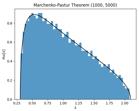
To help visualize the Marchenko-Pastur theorem, Figure 1 displays together

• The eigenvalue density of the empirical correlation matrix of a $n = 1000$ by $T = 5000$ random observation matrix made of i.i.d. standard gaussian variables
• The Marchenko-Pastur density with parameters $q = \frac{1000}{5000} = 0.2$ and $\sigma^2=1$

Figure 1. Eigenvalue density of a $(1000,1000)$ random correlation matrix v.s. its associated Marchenko-Pastur density $(0.2,1)$.

A couple of remarks to finish:

• The parameter $q$ is usually called the aspect ratio of the empirical covariance matrix $\Sigma$
• When $q > 1$, the Marchenko-Pastur theorem is still valid¹, with an additional Dirac mass appearing at $\lambda = 0$ in the Marchenko-Pastur density to account for the null eigenvalues of $\Sigma$

The Marchenko-Pastur theorem in non-asymptotic regime

Because empirical covariance matrices are of finite dimensions in practice, a natural question to ask is whether the Marchenko-Pastur theorem remains applicable in a non-asymptotic regime⁷.

Figure 1 already demonstrates a pretty good agreement between theory and practice with values of $n = 1000$ and $T = 5000$ that are far from infinity.

What about smaller values?

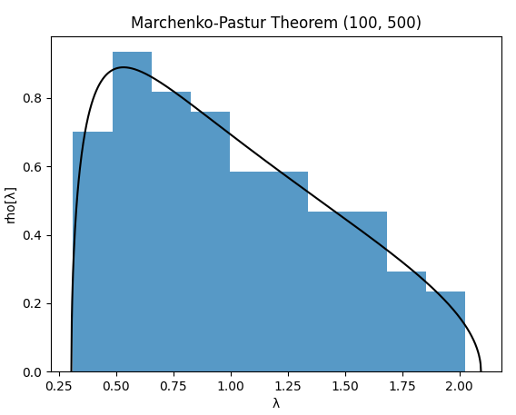
Like $n = 100$ and $T = 500$, displayed in Figure 2.

Figure 2. Eigenvalue density of a $(100,100)$ random correlation matrix v.s. its associated Marchenko-Pastur density $(0.2,1)$.

Or even like $n = 10$ and $T = 50$, displayed in Figure 3.

Figure 3. Eigenvalue density of a $(10,10)$ random correlation matrix v.s. its associated Marchenko-Pastur density $(0.2,1)$.

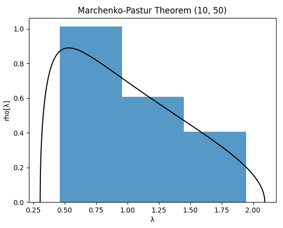
Based on Figures 1 to 3, it appears that the Marchenko-Pastur theorem remains applicable with small values of $n$ and $T$ down to $\approx 100$, but that caution is warranted for very small values of $n$ and $T$ of order $\approx 10$.

More on this later.

A method to denoise correlation matrices based on random matrix theory

Description

Laloux et al.² propose a method to denoise empirical correlation matrices based on random matrix theory, called the eigenvalues clipping method⁸.

The rationale behind this method is that by comparing the spectrum of an empirical correlation matrix to the spectrum of a random correlation matrix it is possible to identify the random part of the empirical correlation matrix.

More formally, let be:

• $C \in \mathcal{M}(\mathbb{R}^{n \times n})$ an empirical correlation matrix associated to a (large) universe of $n$ variables, determined using $T > n$ observations per variable.
• $\lambda_1 \ge \lambda_2 \ge … \ge \lambda_n \ge 0$ the eigenvalues of $C$
• $0 < q = \frac{n}{T} < 1$

Then, the upper edge $\lambda_{+}$ of the Marchenko-Pastur density can serve as a threshold to identify the noisy part of $C$:

• All the eigenvalues of $C$ belonging to $[\lambda_{-}, \lambda_{+}]$ are compatible with the hypothesis of a random correlation matrix and can be considered to represent eigenvalues associated to noise
• All the eigenvalues of $C$ strictly smaller than $\lambda_{-}$ can also be considered to represent eigenvalues associated to noise⁹
• All the eigenvalues of $C$ strictly greater than $\lambda_{+}$ are not compatible with the hypothesis of a random correlation matrix and can be considered to represent “true” eigenvalues

This leads to the following method to denoise $C$:

• All the eigenvalues of $C$ lower than or equal to $\lambda_{+}$ are replaced by a constant value
  • Either equal to the average value of the “noisy” eigenvalues, as in the original paper of Laloux et al.²
  • Or equal to zero, as in Plerou et al.¹⁰¹¹
• All the eigenvalues of $C$ strictly greater than $\lambda_{+}$ are left unchanged

The reason why the eigenvalues associated to noise should be replaced by a constant value is that²

Since the eigenstates corresponding to the “noise band” are not expected to contain real information, one should not distinguish the different eigenvalues […] in this sector.

Practical details

Two important practical details are missing from the previous description of the eigenvalues clipping method.

$q$ must be an adjustable parameter

Comparing an empirical correlation matrix of aspect ratio $q$ to a random correlation matrix of aspect ratio $q$ is usually incorrect because of the presence of both temporal correlations (auto-correlations) and spatial correlations (cross-sectional correlations) in the observations used to estimate the empirical correlation matrix¹.

This is especially true for time series of asset returns².

As a consequence, the aspect ratio $q$ must be considered as an adjustable parameter and not as a constant value equal to $\frac{n}{T}$, as explained by Potters and Bouchaud¹

Intuitively, correlated samples are somehow redundant and the sample [correlation] matrix should behave as if we had observed not $T$ samples but an effective number $T^* < T$.

$\sigma^2$ must be an adjustable parameter

Comparing an empirical correlation matrix to a purely random correlation matrix is also usually incorrect, because empirical eigenvalues strictly above $\lambda_{+}$ are reducing the variance $\sigma^2$ of the random part of the empirical correlation matrix².

This variance must then be considered as an adjustable parameter and not as a constant value equal to one.

Finding the best values of the adjustable parameters $q$ and $\sigma^2$

Because of what precedes, the eigenvalues clipping method must in practice include a preliminary step to find the “best” values of the parameters $q$ and $\sigma^2$, which could for example be defined as the values that bring the eigenvalue density of the random correlation matrix as close as possible¹² to the eigenvalue density of the empirical correlation matrix, as in de Prado¹³.

Figure 4 and Figure 5, taken from Gatheral¹⁴, illustrate the impact of such a preliminary step on the empirical correlation matrix of $n = 431$ stocks belonging to the S&P 500 index and computed using $T = 2,155$ daily returns for each stock¹⁵.

Figure 4. Eigenvalue density of the empirical correlation matrix of the S&P 500 stocks v.s. Marchenko-Pastur density with parameters $(0.2,1)$. Source: Gatheral.

Figure 5. Eigenvalue density of the empirical correlation matrix of the S&P 500 stocks v.s. Marchenko-Pastur density with parameters $(0.34, 0.53)$. Source: Gatheral.

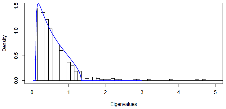
The Marchenko-Pastur density with optimal parameters $q = 0.34$ and $\sigma^2 = 0.53$ displayed on Figure 5 definitely better fits the random part of the eigenvalue density of the empirical correlation matrix than the Marchenko-Pastur density with “by the book” parameters $q = 0.2$ and $\sigma^2 = 1$ displayed on Figure 4.

Implementation in Portfolio Optimizer

Portfolio Optimizer implements the eigenvalues clipping method through the endpoint /assets/correlation/matrix/denoised, using a proprietary algorithm to find the best values of the adjustable parameters $q$ and $\sigma^2$.

Caveats

There is one well-known limitation to the eigenvalues clipping method.

Results from random matrix theory establish that the spectrum of an empirical correlation matrix is usually a broadened version of the spectrum of its true unobservable counterpart⁸. That is, small empirical eigenvalues are usually too small and large empirical eigenvalues are usually too large.

The eigenvalues clipping method does increase the small empirical eigenvalues, but does not alter the large empirical eigenvalues so that they remain overestimated in the denoised empirical correlation matrix.

Example of application - Mean-variance analysis

Markowitz’s mean-variance analysis is one of the most well-known frameworks to construct a portfolio with an optimal level of risk¹⁶ and return from a universe of risky assets.

One of its inputs is a correlation matrix, representing future asset correlations, and while the most natural choice [for it] is to use the sample [correlation] matrix determined using a series of past returns, […] [this choice] […] can lead to disastrous results¹.

Indeed, because the sample correlation matrix is affected by noise, its usage leads to a dramatic underestimation of the real risk, by overinvesting in artificially low-risk eigenvectors¹⁷.

A possible solution to this issue is to denoise it thanks to the eigenvalues clipping method, for which I will illustrate the behaviour on two very different universe of assets.

Large universe of similar assets

Laloux et al.¹⁷ analyze the impact of using the sample correlation matrix v.s. the denoised sample correlation matrix in a large universe of $n = 406$ stocks belonging to the S&P 500 index.

In details, they:

• Split their dataset of stock returns covering the whole period 1991-1996 into two datasets covering respectively the period 1991-1993 and the period 1994-1996.
• Compute¹⁸:
  • A first predicted mean-variance efficient frontier, using as input the sample correlation matrix of the stock returns over the “past” period 1991-1993
  • A second predicted mean-variance efficient frontier, using as input the same sample correlation matrix as before but this time denoised thanks to the eigenvalues clipping method
  • A realized mean-variance efficient frontier, computed using as input the sample correlation matrix of the stock returns over the “future” period 1994-1996

The three resulting efficient frontiers are displayed in Figure 6, taken from Laloux et al.¹⁷, where:

• The leftmost curve represents the first predicted mean-variance efficient frontier
• The middle curve represents the second predicted mean-variance efficient frontier
• The rightmost curve represents the realized mean-variance efficient frontier

Figure 6. Impact of the asset correlation matrix on mean-variance efficient frontiers. Source: Laloux et al.

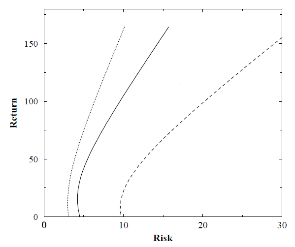
It is clearly visible that:

• The realized risk is underestimated by the two predicted mean-variance efficient frontiers, because the realized mean-variance efficient frontier is located to the left of the two predicted mean-variance efficient frontiers
• The denoised sample correlation matrix is better at predicting the realized risk than the sample correlation matrix, because the second predicted mean-variance efficient frontier is closer to the realized mean-variance efficient frontier than the first one

Large universe of similar assets, part 2

The catch with the previous example¹⁹ is that the predicted mean-variance efficient frontiers are usually computed in the literature without taking into account the real-life constraints faced by individuals or mutual funds like no short sales constraints or maximum investment constraints.

Problem is, Jagannathan and Ma²⁰ established that such constraints have a shrinkage-like effect on the sample asset correlation matrix, very similar to the effect of a denoising method.

As a consequence, the eigenvalues clipping method might actually have no additional value compared to simply imposing asset weight constraints.

In order to determine whether this is the case, I used Portfolio Optimizer to reproduce the methodology of Laloux et al.¹⁷ in a universe of $n = 470$ stocks belonging to the S&P 500 index²¹ and I imposed non-negativity constraints on the computed efficient portfolios’ weights.

The three resulting efficient frontiers are displayed in Figure 7, on which the denoised sample correlation matrix is again visibly better at predicting the realized risk than the sample correlation matrix.

Figure 7. Predicted efficient frontiers v.s. realized efficient frontier for 470 stocks belonging to the S&P 500 index, with non-negativity constraints.

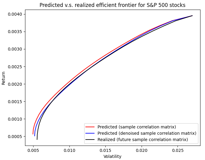
Nevertheless, the improvement is not as dramatic as in Laloux et al.¹⁷, which is in agreement, for example, with the findings of Golden and Flint²² for the South African equity market.

Small universe of dissimilar assets

I will now analyze the impact of using the sample correlation matrix v.s. the denoised sample correlation matrix in the small universe of $n = 10$ assets of the Adaptative Asset Allocation strategy from ReSolve Asset Management, described in the paper Adaptive Asset Allocation: A Primer²³:

• U.S. stocks (SPY ETF)
• European stocks (EZU ETF)
• Japanese stocks (EWJ ETF)
• Emerging markets stocks (EEM ETF)
• U.S. REITs (VNQ ETF)
• International REITs (RWX ETF)
• U.S. 7-10 year Treasuries (IEF ETF)
• U.S. 20+ year Treasuries (TLT ETF)
• Commodities (DBC ETF)
• Gold (GLD ETF)

For this, I propose to adapt the methodology of Laloux et al.¹⁷ to the rules of the Adaptative Asset Allocation strategy²⁴, which leads to the computation of the following quantities at the end of the last trading day of each month:

1. Mean-variance input estimation
   • The past sample correlation matrix $C_i$ of the daily asset returns over the past 6 months ($T \approx 126$)
   • The denoised past sample correlation matrix $\hat{C_i}$, using the Portfolio Optimizer endpoint /assets/correlation/matrix/denoised
   • The future sample correlation matrix $C_o$ of the daily asset returns over the next month
   • The future volatilities $\sigma_o$ of the daily asset returns over the next month
   • The future average returns $\mu_o$ of the daily asset returns over the next month
2. Mean-variance efficient frontiers computation, with a no-short-sales constraint
   • The predicted in-sample mean-variance efficient frontier, using as inputs $\sigma_o$, $C_i$ and $\mu_o$
   • The predicted filtered in-sample mean-variance efficient frontier, using as inputs $\sigma_o$, $\hat{C_i}$ and $\mu_o$
   • The realized out-of-sample mean-variance efficient frontier, using as inputs $\sigma_o$, $C_o$ and $\mu_o$

When applied to the period June 2020 - September 2022²⁵, the results are that:

• ~60% of the time, the two predicted in-sample mean-variance efficient frontiers are nearly indistinguishable, as illustrated in Figure 8

Figure 8. Indistinguishable predicted efficient frontiers v.s. realized efficient frontier.

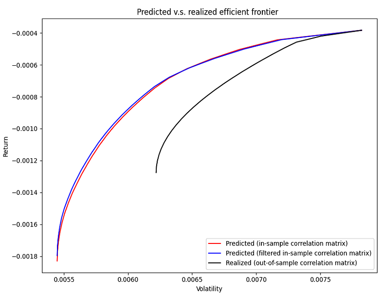
• ~30% of the time, the predicted filtered in-sample mean-variance efficient frontier is slightly closer to realized out-of-sample mean-variance efficient frontier than the predicted in-sample mean-variance efficient frontier, as illustrated in Figure 9

Figure 9. Predicted efficient frontiers v.s. realized efficient frontier, filtered in-sample better than in-sample.

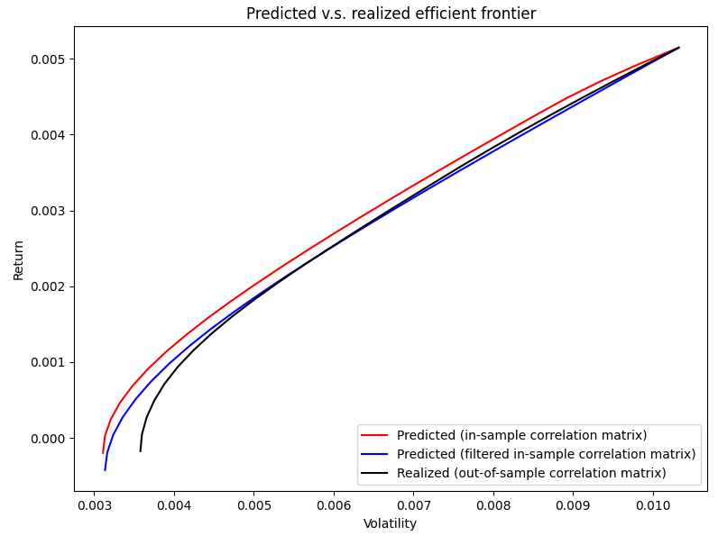
• ~10% of the time, the predicted filtered in-sample mean-variance efficient frontier is slightly farther from the realized out-of-sample mean-variance efficient frontier than the predicted in-sample mean-variance efficient frontier, as illustrated in Figure 10

Figure 10. Predicted efficient frontiers v.s. realized efficient frontier, filtered in-sample worse than in-sample.

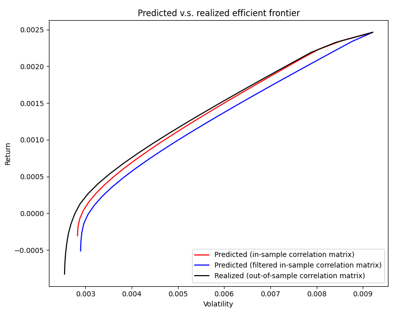
To summarize, on this example, using the denoised sample correlation matrix instead of the sample correlation matrix does no harm or improves the realized risk estimate ~90% of the time²⁶, which is quite remarkable for such small values of $n$ and $T$!

Conclusion

As usual, feel free to connect with me on LinkedIn or to follow me on Twitter if you would like to discuss about Portfolio Optimizer (new feature request, support request…) or random finance stuff.

–

1. See Marc Potters, Jean-Philippe Bouchaud, A First Course in Random Matrix Theory, Cambridge University Press. ↩ ↩² ↩³ ↩⁴ ↩⁵ ↩⁶ ↩⁷ ↩⁸

2. See Laurent Laloux, Pierre Cizeau, Jean-Philippe Bouchaud, and Marc Potters, Noise Dressing of Financial Correlation Matrices, Phys. Rev. Lett. 83, 1467. ↩ ↩² ↩³ ↩⁴ ↩⁵ ↩⁶ ↩⁷

3. When $\sigma^2 = 1$, the matrix $\Sigma$ is the empirical correlation matrix associated to $X$. ↩

4. See V. A. Marchenko, L. A. Pastur - Distribution of eigenvalues for some sets of random matrices - Mat. Sb. (N.S.), 72(114):4 (1967), 507–536. ↩

5. See Pavel Yaskov, A short proof of the Marchenko–Pastur theorem, Comptes Rendus Mathematique Volume 354, Issue 3, March 2016. ↩

6. Under the proper technical assumptions mentioned above. ↩

7. Which could not be the case, for example because of an extremely slow rate of convergence. ↩

8. See Joel Bun, Jean-Philippe Bouchaud, Marc Potters, Cleaning correlation matrices, Risk.net. ↩ ↩²

9. This is not a theoretical consequence of the Marchenko-Pastur theorem, but rather a practical consequence of the attempt to limit small eigenvalues. In addition, small eigenvalues are usually not as clearly separated from the bulk of the spectrum as the large eigenvalues. ↩

10. See Vasiliki Plerou, Parameswaran Gopikrishnan, Bernd Rosenow, Luís A. Nunes Amaral, Thomas Guhr, and H. Eugene Stanley, Random matrix approach to cross correlations in financial data, Phys. Rev. E 65, 066126, 27 June 2002. ↩

11. Choosing the constant equal to zero requires an additional manipulation of the denoised correlation matrix to make it a valid correlation matrix, c.f. Plerou et al.¹⁰. ↩

12. For example, in terms of $l^2$ norm. ↩

13. See Lopez de Prado, Marcos, A Robust Estimator of the Efficient Frontier. ↩

14. See Jim Gatheral, Random Matrix Theory and Covariance Estimation, NYU Courant Institute Algorithmic Trading Conference (October 2008). ↩

15. The aspect ratio of this empirical correlation matrix is thus $q = \frac{431}{2,155} = 0.2$. ↩

16. In mean-variance analysis, the risk of a portfolio is defined in terms of the variance of its returns. ↩

17. See Laurent Laloux, Pierre Cizeau, Jean-Philippe Bouchaud, and Marc Potters, Random matrix theory and financial correlations, International Journal of Theoretical and Applied Finance, Vol. 03, No. 03, pp. 391-397 (2000). ↩ ↩² ↩³ ↩⁴ ↩⁵ ↩⁶

18. In order to isolate the impact of the asset correlations from the asset returns and the asset volatilities, future asset returns and future asset volatilities are used in the computation of the efficient frontiers. ↩

19. For example, the same remark applies to Plerou et al.¹⁰. ↩

20. See Ravi Jagannathan & Tongshu Ma, 2003. Risk Reduction in Large Portfolios: Why Imposing the Wrong Constraints Helps, Journal of Finance, American Finance Association, vol. 58(4), pages 1651-1684, 08. ↩

21. The associated dataset, which covers the period 11th February 2013 - 07th February 2018, is available on Kaggle. ↩

22. See Golden, Daron and Flint, Emlyn, Improving Portfolio Allocation Through Covariance Matrix Filtering. ↩

23. See Butler, Adam and Philbrick, Mike and Gordillo, Rodrigo and Varadi, David, Adaptive Asset Allocation: A Primer. ↩

24. Taken from Allocate Smartly’s blog. ↩

25. I retrieved the adjusted ETF prices over the period January 2020 - September 2022 using Tiingo. ↩

26. A possible next step would be to determine if this improves the backtested performances of the Adaptative Asset Allocation strategy. ↩