The Matrix Effective Rank: Measuring the Dimensionality of a Universe of Assets
Quantifying how diversified is a universe of assets is an open problem in quantitative finance, partly because there is no definite formula for diversification1.
Let’s make the (reasonable) assumption that the way assets are moving together within a universe is important for its diversification.
This in turn makes asset correlations within a universe important in determining how diversified it is.
For example, consider the following correlation matrices:
\[C_1 = \begin{bmatrix} 1 & 0 & 0 \newline 0 & 1 & 0 \newline 0 & 0 & 1 \end{bmatrix}\] \[C_2 = \begin{bmatrix} 1 & 1 & 0 \newline 1 & 1 & 0 \newline 0 & 0 & 1 \end{bmatrix}\] \[C_3 = \begin{bmatrix} 1 & 0.99 & 0.98 \newline 0.99 & 1 & 0.99 \newline 0.98 & 0.99 & 1 \end{bmatrix}\]Intuitively, $C_1$, $C_2$ and $C_3$ are describing asset correlations within 3 very different universe of 3 assets:
- $C_1$ represents a universe made of 3 different assets
- $C_2$ represents a universe made of only 2 different assets2
- $C_3$ represents a universe made of essentially 1 asset3
So, question is, would it be possible to “transform” an asset correlation matrix into a measure of diversification for the associated universe?
The matrix effective rank, introduced by Roy and Vetterli4 as a real-valued extension of the matrix rank with roots in information theory, can be used in this context.
Indeed, the effective rank of $C_1$, $C_2$ and $C_3$ matches quite closely the intuition above:
- The effective rank of $C_1$ is equal to 3
- The effective rank of $C_2$ is equal to ~1.89
- The effective rank of $C_3$ is equal to ~1.06
In this post, after providing the formal definition of the matrix effective rank and some of its properties, I will illustrate one of its possible usage in principal components analysis.
Notes:
- A Google sheet corresponding to this post is available here
Mathematical preliminaries
Definition
Let be:
- $A \in \mathcal{M}(\mathbb{R}^{n \times n})$, $n \ge 2$, a non null real symmetric positive semi-definite matrix
- $\lambda_1 \ge \lambda_2 \ge … \ge \lambda_n \ge 0$ the eigenvalues of the matrix $A$5
- $\rho_1 \ge \rho_2 \ge … \ge \rho_n \ge 0$ the standardized eigenvalues of the matrix $A$ defined by $\rho_i = \frac{\lambda_i}{\sum_{i=1}^{n} \lambda_i}$, $i=1..n$
The effective rank of the matrix $A$ is defined as the exponential Shannon entropy of its standardized eigenvalues6, that is
\[\textrm{erank}(A) = e^{- \sum_{i=1}^{n} \rho_i \ln(\rho_i)}\]Interpretation
The well known matrix rank corresponds to the (algebraic) dimension of the vector space generated by the columns of a matrix - the matrix range - and does not take into account the actual geometry of this vector space.
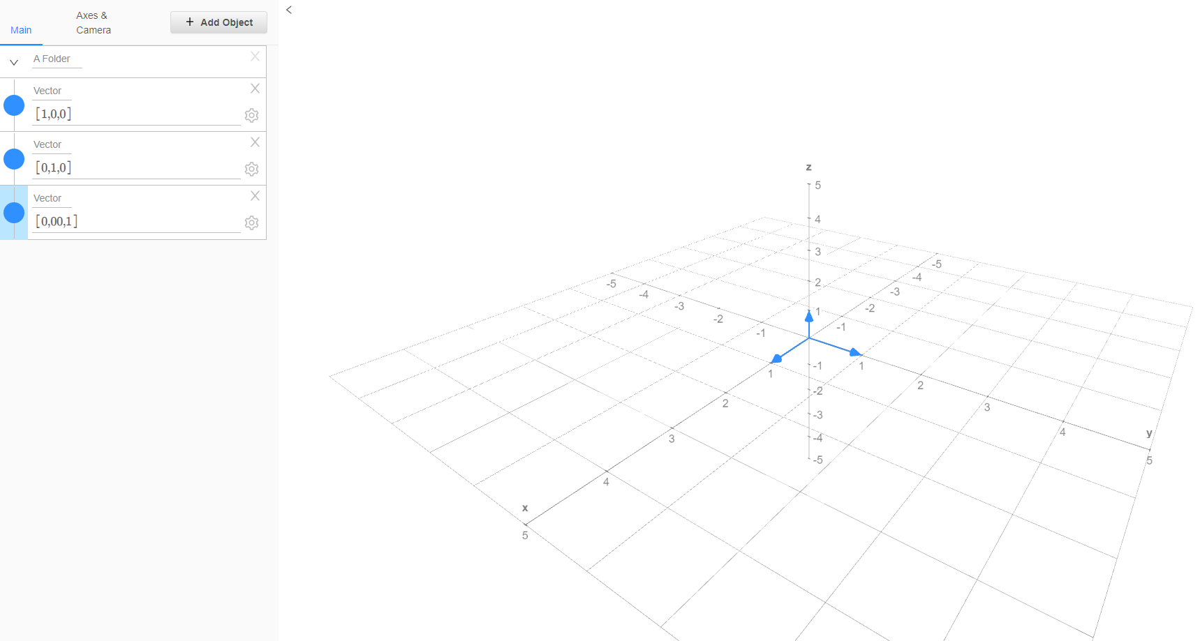
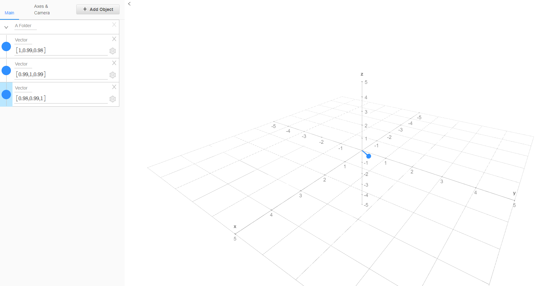
For example, both matrices $C_1$ and $C_3$ are of rank 3, so that their range is $\mathbb{R}^3$, but:
- The range of $C_1$ is geometrically identical to $\mathbb{R}^3$, as illustrated on Figure 1

- The range of $C_3$ is geometrically close to a line in $\mathbb{R}^3$, as illustrated on Figure 2

On the other hand, the matrix effective rank is directly influenced by the geometrical shape of the matrix range4 and represents the true, effective, dimension of this vector space.
Thus, when computed on an asset correlation (or covariance) matrix, the effective rank measures the dimensionality of the associated universe of assets.
Main properties
Below are the main properties of the matrix effective rank established in Roy and Vetterli4.
Let $A, B \in \mathcal{M}(\mathbb{R}^{n \times n})$, $n \ge 2$, be two non null real symmetric positive semi-definite matrices.
Property 1: $1 \le \textrm{erank}(A) \le \textrm{rank}(A) \le n$
Property 2: $\textrm{erank}(A)$ takes all the values in the real interval $[1, \textrm{rank}(A)]$
Property 3: $\textrm{erank}(A) = \textrm{erank}(A {}^t)$
Property 4: $\textrm{erank}(A+ B) \le \textrm{erank}(A) + \textrm{erank}(B)$
The matrix effective rank as a diversity index
One interesting connection to make is that in the domain of biology7, the matrix effective rank actually corresponds to a diversity index called the Hill number of order 1.
Example of usage - Principal components analysis (PCA)
As an illustration of a possible usage, I will reproduce the results of Fleming and Kroeske8 about the explanatory power of the number of components indicated by the matrix effective rank in principal components analysis.
Data
Fleming and Kroeske8 use daily and weekly closing prices of assets belonging to 3 different universes9 over the period 1992 - 2012.
In this post, I use monthly closing prices10 of the Sector SPDR ETFs11 over the period 2000 - 202112.
Methodology
Similar to Fleming and Kroeske8, I use a rolling window approach.
At the end of each month:
- The covariance matrix $\Sigma$ of the ETFs is computed over the previous 24 months of ETF returns data13, using the Portfolio Optimizer endpoint
/assets/covariance/matrix/estimation/empirical - The effective rank of $\Sigma$ is determined, using the Portfolio Optimizer endpoint
/assets/covariance/matrix/effective-rank - The principal components of $\Sigma$ are determined, using the Portfolio Optimizer endpoint
/portfolio/analysis/factors/implicit - The proportion of the total variance explained by the $\left \lceil{\textrm{erank}(A)}\right \rceil$ principal components of $\Sigma$ is computed
Results
The results obtained are remarkably consistent with those of Fleming and Kroeske8:
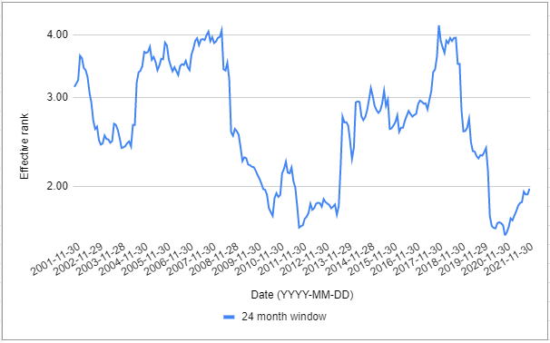
- The effective rank varies a lot through time14, as illustrated on Figure 3

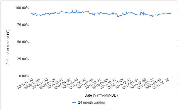
- The proportion of total variance explained is both very high and very stable through time15, as illustrated on Figure 4

Conclusion
I hope you enjoyed this first post of 2022!
Another possible usage of the matrix effective rank, hinted in Fleming and Kroeske8, is to use it as an indicator of systemic risk.
Indeed, it appears that the matrix effective rank bottoms around market crashes (financial crisis of 2007–2008, Corona crisis of 2020…).
Maybe a subject for another time…
–
-
See Meucci, Attilio, Managing Diversification (April 1, 2010). Risk, pp. 74-79, May 2009, Bloomberg Education & Quantitative Research and Education Paper. ↩
-
The first asset and the second asset are moving in sync, and so are identical from a diversification perspective. ↩
-
The matrix $C_3$ is a small perturbation of the equicorrelation matrix $\begin{bmatrix} 1 & 1 & 1 \newline 1 & 1 & 1 \newline 1 & 1 & 1 \end{bmatrix}$ which represents a universe where all the assets are moving in sync. ↩
-
See Olivier Roy and Martin Vetterli, The effective rank: A measure of effective dimensionality, 15th European Signal Processing Conference, 2007. ↩ ↩2 ↩3
-
The eigenvalues of a non null real symmetric positive semi-definite matrix are all real, non-negative and at least one of them is strictly positive. ↩
-
With the convention that $0 \ln(0) = 0$. ↩
-
See Jost, L. (2006), Entropy and diversity. Oikos, 113: 363-375. ↩
-
See Fleming, Brian and Kroeske, Jens, An Information-Theoretic Approach to Dimension Reduction of Financial Data (June 3, 2013). ↩ ↩2 ↩3 ↩4 ↩5
-
U.K. spot government bond yields across 13 maturities, 66 U.S. equity industries and 96 multi-asset class data series including equities, government bonds, corporate bonds, currencies and commodities. ↩
-
Adjusted for splits and dividends. ↩
-
Provided by Alpha Vantage. ↩
-
As they become available through time. ↩
-
The 24 months of data correspond to the 2 years of data used by Fleming and Kroeske8. ↩
-
Ranging from ~1.60 to ~4.18. ↩
-
Ranging from ~87% to ~96%. ↩