Beyond Hierarchical Risk Parity: Hierarchical Clustering-Based Risk Parity
In a previous post, I introduced the Hierarchical Risk Parity portfolio optimization algorithm1.
In this post, I will present one of its variations, called Hierarchical Clustering-Based Risk Parity, first described in Papenbrock2 and then generalized in Raffinot34 and in Lohre et al.5, from which the implementation in Portfolio Optimizer is inspired.
Hierarchical clustering-based risk parity algorithm overview
Step 1 - Hierarchical clustering of the assets
The Hierarchical Clustering-Based Risk Parity algorithm builds onto the Hierarchical Risk Parity algorithm in that its first step also consists in using a hierarchical clustering algorithm to group similar assets together.
Now, there are a few differences:
- Instead of single linkage, the linkage method used is Ward’s linkage in order to avoid suffering from the chaining effect and also to produce compact clusters of similar size
- Instead of being correlation-based, the similarity measure used can be of any sort, for example based on lower tail dependence5, in order to try to capture different properties
- Instead of being executed until each asset is in its own cluster, the hierarchical clustering algorithm is stopped as soon as a predefined number of clusters has been computed in order to avoid overfitting the data
The impact on the shape of the dendrogram of using different linkage methods is illustrated in Figure 1, taken from Lohre et al.5:

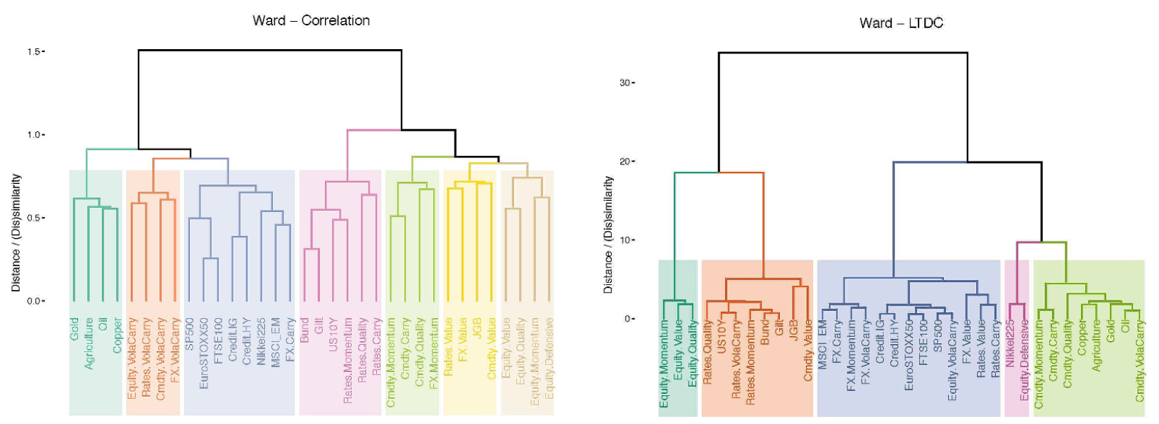
The impact on the shape of the dendrogram of using a different similarity measure than the correlation-based similarity measure of the Hierarchical Risk Parity algorithm is illustrated in Figure 2, also taken from Lohre et al.5:
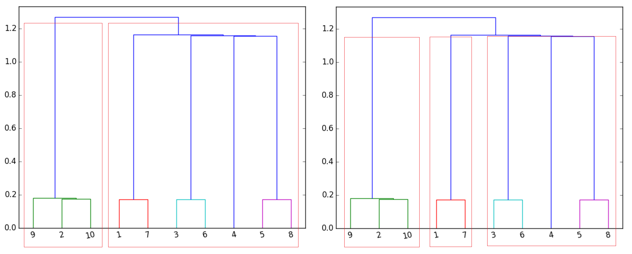
The impact on the shape of the dendrogram of early stopping the hierarchical clustering algorithm is illustrated in Figure 3:
In Portfolio Optimizer:
- 4 linkage methods are supported:
- Single linkage
- Complete linkage
- Average linkage
- (Default) Ward’s linkage
- At the date of the publication of this post, only the correlation matrix is supported as a means to group similar assets together.
- The number of clusters can either be provided by the user or be automatically computed using the gap index method6, as proposed in Raffinot34. In the latter case, the null reference distribution of the data is the uniform distribution over the set of positive definite correlation matrices7.
Step 2 - Top-Down recursive division into two parts based on the dendrogram and assets weights computation
The second step of the Hierarchical Clustering-Based Risk Parity algorithm consists in recursively dividing the hierarchical tree computed in the first step into two parts and, while doing so, computing assets weights using any portfolio optimization algorithm for both the within-cluster and the across-cluster allocations.
This second step of the Hierarchical Clustering-Based Risk Parity algorithm contrasts with the third step of the Hierarchical Risk Parity algorithm, in which the shape of the dendrogram produced by the first step is ignored by the recursive bisection procedure8.
This difference in behavior is illustrated on Figure 4, in which the Hierarchical Risk Parity algorithm is wrongly splitting the two highly correlated assets #2 and #3 in two different clusters, while the Hierarchical Clustering-Based Risk Parity algorithm is properly splitting asset #1 in one cluster and assets #2, #3 and #4 in another cluster.

In Portfolio Optimizer:
- 3 methods for the within and across cluster allocations are supported:
- (Default) Equal weighting9
- Inverse volatility
- Inverse variance
- Minimum and maximum assets weights constraints are supported thanks to a variation of the method described in Pfitzinger et al.10.
Hierarchical clustering-based risk parity algorithm usage with Portfolio Optimizer
As a quick practical example of Portfolio Optimizer usage, I propose to reproduce the exhibit 1 of Raffinot3, represented on Figure 5.
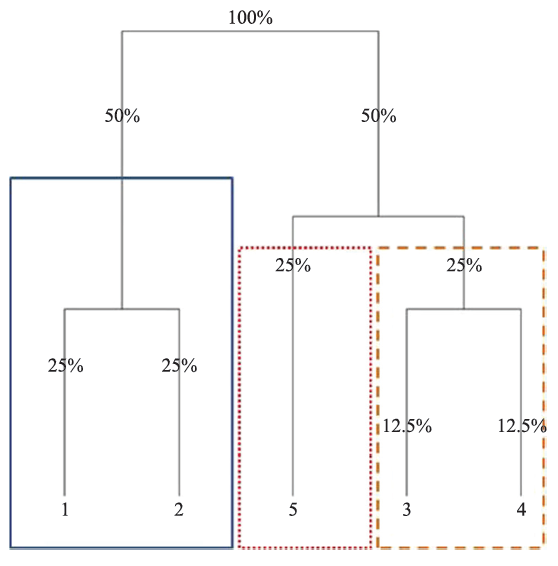
Figure 5 represents a universe of 5 assets with a covariance matrix equal to $\begin{bmatrix} 1 & 1 & 0 & 0 & 0 \newline 1 & 1 & 0 & 0 & 0 \newline 0 & 0 & 1 & 0 & 0 \newline 0 & 0 & 0 & 1 & 1 \newline 0 & 0 & 0 & 1 & 1 \end{bmatrix}$ and with a dendrogram restricted to 3 clusters.
In order to compute the associated assets weights, it suffices to call the Portfolio Optimizer endpoint /portfolios/optimization/hierarchical-risk-parity/clustering-based with the following input data:
This results in the following output, which matches with the expected assets weights displayed on Figure 5:
{
  "assetsWeights": [0.25, 0.25,0.25,0.125,0.125]
}
Last words
Feel free to reach out if you need to outsource any portfolio optimization algorithm, or if you would like support in integrating Portfolio Optimizer!
–
-
See Lopez de Prado, M. (2016). Building diversified portfolios that outperform out-of-sample. Journal of Portfolio Management, 42(4), 59–69. ↩
-
See Papenbrock, Jochen, Asset Clusters and Asset Networks in Financial Risk Management and Portfolio Optimization. ↩
-
See Thomas Raffinot, Hierarchical Clustering-Based Asset Allocation, The Journal of Portfolio Management Multi-Asset Special Issue 2018, 44 (2) 89-99. ↩ ↩2 ↩3
-
See Thomas Raffinot, The Hierarchical Equal Risk Contribution Portfolio. ↩ ↩2
-
See Machine Learning for Asset Management: New Developments and Financial Applications, Emmanuel Jurczenko, Chapter 9, Harald Lohre, Carsten Rother, Kilian Axel Schäfer, Hierarchical Risk Parity: Accounting for Tail Dependencies in Multi-asset Multi-factor Allocations. ↩ ↩2 ↩3 ↩4
-
See Tibshirani, R., G. Walther, and T. Hastie. “Estimating the Number of Clusters in a Data Set via the Gap Statistic.” Journal of the Royal Statistical Society: Series B (Statistical Methodology), Vol. 63, No. 2 (2001), pp. 411-423.. ↩
-
The generation of correlation matrices uniformly at random over the space of positive definite correlation matrices is done thanks to a computationally more efficient version of the partial correlations method described in Joe, H., Generating random correlation matrices based on partial correlations. Journal of Multivariate Analysis, 2006, 97, 2177-2189. ↩
-
The recursive bisection procedure of the Hierarchical Risk Parity algorithm only takes into account the order of the leaves of the dendrogram. ↩
-
Using Equal weighting for both within and across cluster allocation methods corresponds to the Hierarchical Clustering-Based Asset Allocation (HCAA) described in Raffinot3. ↩
-
See Johann Pfitzinger & Nico Katzke, 2019. A constrained hierarchical risk parity algorithm with cluster-based capital allocation. Working Papers 14/2019, Stellenbosch University, Department of Economics. ↩