The Market Rank Indicator: Measuring Financial Risk, Part 3
In the previous post of this series on measuring financial risk, I described the absorption ratio, a measure of financial market fragility based on principal components analysis, introduced in Kritzman et al.1.
In this new blog post, I will describe another measure of financial distress called the market rank indicator (MRI), this time related to the notion of condition number2 of a matrix, introduced in Figini et al.2.
As an example of usage, I will show how to use the market rank indicator to dynamically scale the market exposure of a portfolio of U.S. equities.
The market rank indicator
Definition
Let be:
- $n$, the number of assets
- $T$, the number of time periods, with $T > n$
- $X \in \mathbb{R}^{T \times n}$, the matrix of the asset arithmetic or logarithmic returns for each of the $T$ time periods
- $\sigma_1,…,\sigma_n$, the singular values of $X$ ordered such that $0 < \sigma_1 \leq … \leq \sigma_n$
- $1\leq k \leq n$, the number of singular values $\lambda_1,…,\lambda_k$ to retain in the computation of the market rank indicator
The market rank indicator $\text{MRI}$ of the assets is defined2 as the ratio between the largest singular value and the geometric mean of the $k$ smallest singular values of the matrix $X$2, that is
\[\text{MRI}_k = \frac{ \sigma_n }{ \left( \prod_{i=1}^k \sigma_i \right)^{1/k} }\]Alternative definition
Let be:
- $n$, the number of assets
- $T$, the number of time periods, with $T > n$
- $X \in \mathbb{R}^{T \times n}$, the matrix of the asset arithmetic or logarithmic returns for each of the $T$ time periods
- $\Sigma = \frac{1}{T} X {}^t X \in \mathcal{M}(\mathbb{R}^{n \times n})$, the asset returns covariance matrix
- $\lambda_1,…,\lambda_n$, the eigenvalues of $\Sigma$ ordered such that $0 < \lambda_1 \leq … \leq \lambda_n$
Thanks to the relationship $\lambda_i = \frac{\sigma_i^2}{T}$, $i=1..n$, between the eigenvalues of $\Sigma$ and the singular values of $X$, the market rank indicator can alternatively be defined as the square root of the ratio between the largest eigenvalue and the geometric mean of the $k$ smallest eigenvalues of the matrix $\Sigma$, that is
\[\text{MRI}_k = \sqrt{ \frac{ \lambda_n }{ \left( \prod_{i=1}^k \lambda_i \right)^{1/k} } }\]Generalized definition
In the two previous sub-sections, it is assumed that $T > n$.
This is to guarantee that the singular values of the matrix $X$ or that the eigenvalues of the matrix $\Sigma$ are not null.
In case $T \leq n$, the definition of the market rank indicator needs to be adapted, which is simply done by redefining [it] on the first $T$ [non zero] singular values2.
Rationale
Figini et al.2 highlights that what contains valuable information on market synchronization in a principal components analysis on asset returns is not only the strength of the first principal component, but also the weakness of the last components2.
This observation leads to the proposal of the market rank indicator as a generalization of the condition number $\kappa(X)$ of the matrix $X$2, with $\text{MRI}_1 = \kappa(X)$ as a special case.
Interpretation
Figini et al.2 proposes both a mathematical and a financial interpretation of the market rank indicator:
-
Mathematically, the market rank indicator measures the difficulty to span $\mathbb{R}^n$ with the $n$ columns of $X$2.
Indeed, for a given $1\leq k \leq n$, a large value of $\text{MRI}_k$ indicates that […] the columns of $X$ are a basis for an $(n − k)$-dimensional space2.
-
Financially, the market rank indicator may be interpreted as a measure of distance of the asset return series from a market where the number of independent assets is reduced2.
Indeed, again for a given $1\leq k \leq n$, a large value of $\text{MRI}_k$ indicates that $k$ dimensions/assets out of $n$ are not very useful in diversifying a portfolio2.
Theoretical and empirical properties
Figini et al.2 establishes several theoretical properties of the market rank indicator, among which:
Property 1: For any $1 \leq k \leq n$, $ 1 \leq \text{MRI}_k \leq \text{MRI}_1 $.
Property 2: For a given matrix $X$, $\text{MRI}_k$ is non-increasing in $1 \leq k \leq n$.
In addition, Figini et al.2 empirically demonstrates that the market rank indicator is a suitable early warning system for future turbulence on the market2 by showing3 that a large value of [that indicator] signals that the market will experience worse performances in the near future and that the probability of a large and negative return increases2.
How to determine the number of singular values to retain?
When computing the market rank indicator, Figini et al.2 suggests to use a number of singular values of about 1/3th the number of assets2:
The value for $k$ is set after a careful sensitivity analysis: an extensive comparison of the results obtained under different parameter settings showed that the best choice for $k$ is around one third of $n$.
To be noted, though, that depending on the specific context at hand, the number of singular values to retain could also be chosen using the numerical optimization method, assuming for example $k$ stochastic2.
Comparison with other measures of financial risk
Comparison with the absorption ratio
Figini et al.2 notes that critical market conditions2 are characterized by two connected but not perfectly equivalent2 phenomena:
- An increase in the weight of the first principal components2
- A reduction in the weight of the last components2
The absorption ration focuses on the quantity of variability explained by the largest components2, that is, it focuses on the first phenomenon.
The market rank indicator, on the other hand, focuses on the second phenomenon2, which theoretically makes it a perfect complement to the absorption ratio as a measure of financial risk.
Comparison with the covariance matrix effective rank
Familiar readers might remember that in a previous blog post, I discussed the effective rank4 of a covariance matrix, which is a real-valued extension of its rank allowing to measure the dimensionality of the associated universe of assets.
It turns out - as its name suggests - that the market rank indicator is very similar to the effective rank.
Indeed, when there is an increase in the co-movement of the asset returns2, the vectors of the return time series become closer2, which leads to a reduction in the diversification opportunities or, from a numerical point of view, a reduction in the market “dimension”2 which is also captured by the effective rank.
As an illustration, Figure 1 compares both indicators when applied to the 11 Vanguard U.S. sector ETFs5 over the period 31th October 2005 - 30th January 2026, using the same methodology as described in the Exemple of usage section.
On Figure 1, it is clearly visible that the market rank indicator and the effective rank move in a near perfect opposite direction to each other, which is confirmed numerically by a -84% correlation between these two indicators.
Still, the inverse relationship between the market rank indicator and the effective rank is not perfect6, so that they might be considered as two similar-but-different indicators.
Horse race for Value-at-Risk forecasting
Figini et al.2 compares the empirical performances of the market rank indicator to those of three other measures of financial risk (the absorption ratio, the turbulence index and the average correlation) when forecasting the level of the 20-day ahead Value-at-Risk, and shows that it is the indicator which displays the best performances2.
In more details, Figini et al.2:
-
First notes that in general, a good systemic risk indicator would allow to well discriminate between the regular behavior of the market and periods of distress2 because intuitively, the VaR (or other risk indicators) should be low when the indicator is low and large when the indicator is large2.
-
Then proceeds to empirically test this assumption in the case of the S&P 500 index, the STOXX Europe 600 index and the DAX index and concludes that:
Although each indicator presents a degree of forecasting power, the MRI is the indicator which displays the best performances for the three markets.
In fact, [as can be seen in Figure 2] not only the VaR associated to the highest percentile interval is the largest, but also the difference between the VaR associated to the highest interval and the one associated to the lowest interval present the largest outcomes as well […].
This shows that the MRI can best discriminate between regular and turbulent periods, with respect to other systemic risk indicators.
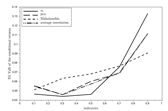
Figure 2. Future 20-day S&P 500 Value-at-Risk at 5% level v.s. quintiles of various systemic risk indicators, 02nd January 1992 - 01st July 2011. Source: Figini et al.
Implementation in Portfolio Optimizer
Portfolio Optimizer implements the computation of the market rank indicator through the endpoint /assets/analysis/market-rank-indicator, with the default number of singular values to retain
suggested in Figini et al.2.
Example of usage - Scaling the market exposure of a portfolio of U.S. equities
I will now illustrate the performances of the market rank indicator in a trading strategy desgined to capture the idea that exposure to stocks should be decreased when the market rank indicator is increasing.
For this:
-
I will work within the universe of U.S. equities represented by the SPY ETF and the 11 Vanguard U.S. sector ETFs5.
-
I will rely on daily return data7 over the period 31th October 2005 - 30th January 2026.
-
I will use the following trading strategy at the end of each month:
- Compute the sample covariance matrix of the 11 Vanguard U.S. sector ETFs over the past month, using the ETF daily arithmetic returns.
- Compute the market rank indicator associated to that covariance matrix, retaining 3 eigenvalues.
- Determine how elevated is this market rank indicator relative to its past 12-month history on a scale $s$ from 0% to 100%, thanks to a percentile rank.
- If $s$ is greater than 75% (i.e., relatively elevated recent market rank indicator), allocate the portfolio to cash (with 0% interest) else allocate the portfolio to U.S. equities (SPY ETF); in both cases, hold that portfolio for the next month.
The equity curve associated to that market rank indicator-based trading stategy is depicted in Figure 3.
From Figure 3, the market rank indicator-based trading stategy does a good job in avoiding some serious drawdowns when compared to the buy and hold strategy, but unfortunately lags in terms of total return.
Figures:
| Portfolio Management Strategy | Average Exposure | CAGR | Annualized Sharpe Ratio | Maximum (Monthly) Drawdown |
|---|---|---|---|---|
| Buy and hold | 100% | 10.9% | 0.78 | 51% |
| MRI-based | 68% | 8.2% | 0.79 | 33% |
For comparison, Figure 4 additionally depicts the equity curve associated to a similar strategy, this time based on the absorption ratio of the 11 Vanguard U.S. sector ETFs8.
With figures:
| Portfolio Management Strategy | Average Exposure | CAGR | Annualized Sharpe Ratio | Maximum (Monthly) Drawdown |
|---|---|---|---|---|
| Buy and hold | 100% | 10.9% | 0.78 | 51% |
| MRI-based | 68% | 8.2% | 0.79 | 33% |
| AR-based | 69% | 10.6% | 1.03 | 21% |
From Figure 4, it seems that that the absorption ratio is superior9 to the market rank indicator in terms of predictive performances for the specific universe of assets and over the specific period considered here.
Incidentally, that result is at odds with the findings of Figini et al.2, so that the interested reader might want to dig deeper…
Conclusion
Together with the turbulence index and the absorption ratio10, the market rank indicator is a simple early warning indicator2 for dangerous periods on financial markets.
Although it did not particularly shine v.s. the absorption ratio in the specific example studied in this blog post, the market rank indicator is definitely an additional tool to integrate2 so as to improve [one’s] warning system2.
Waiting for the analysis of the other measures of financial risk, feel free to connect with me on LinkedIn or to follow me on Twitter.
–
-
See Mark Kritzman, Yuanzhen Li, Sebastien Page and Roberto Rigobon, Principal Components as a Measure of Systemic Risk, The Journal of Portfolio Management Summer 2011, 37 (4) 112-126. ↩
-
See Silvia Figini, Mario Maggi, Pierpaolo Uberti, The market rank indicator to detect financial distress, Econometrics and Statistics, Volume 14, 2020, Pages 63-73. ↩ ↩2 ↩3 ↩4 ↩5 ↩6 ↩7 ↩8 ↩9 ↩10 ↩11 ↩12 ↩13 ↩14 ↩15 ↩16 ↩17 ↩18 ↩19 ↩20 ↩21 ↩22 ↩23 ↩24 ↩25 ↩26 ↩27 ↩28 ↩29 ↩30 ↩31 ↩32 ↩33 ↩34 ↩35 ↩36 ↩37 ↩38 ↩39 ↩40
-
Using returns of the 10 sectors composing the S&P 500 index. ↩
-
See Olivier Roy and Martin Vetterli, The effective rank: A measure of effective dimensionality, 15th European Signal Processing Conference, 2007. ↩
-
These are “VOX”, “VCR”, “VDC”, “VDE”, “VFH”, “VHT”, “VIS”, “VGT”, “VAW”, “VNQ”, “VPU”, c.f. https://investor.vanguard.com/investment-products/etfs/sector-etfs. ↩ ↩2
-
Most probably due to the fact that the number of eigenvalues used by each indicator is different. ↩
-
(Adjusted) prices of the ETFs have have been retrieved using Tiingo. ↩
-
The absorption ratio-based trading strategy is exactly the same as the market rank indicator-based trading strategy, except that the absorption ratio is computed instead of the market rank indicator; that’s the only change. ↩
-
The two indicators are agreeing most of the time - their correlation is 85%; as a side note, it could be interesting to understand what happens when they are disagreeing… ↩
-
As well as the effective rank; I cannot insist too much on that one, though, because - to this date - I did not analyze its usefulness as a measure of financial risk on the blog. ↩