The Mathematics of Portfolio Return: Simple Return, Money-Weighted Return and Time-Weighted Return

Whether we manage our own investment assets or choose to hire others to manage the assets on our behalf we are keen to know how well our […] portfolio of assets is performing¹ and the calculation of portfolio return is the first step in [that] performance measurement process¹.

Now, while the matter of measuring the rate of return of [a portfolio] appears, on the surface, to be simple enough², the presence of external cash flows - either contributions to the portfolio or withdrawals from the portfolio - leads to the definition of several rate of returns, with no single rate of return measure [being] appropriate for every purpose².

In this blog post, strongly inspired by the book Practical Portfolio Performance Measurement and Attribution² from Carl Bacon, I will describe the two main methods of portfolio return calculation in the presence of external cash flows.

As an example of usage, I will illustrate the investor gap in the case of a MSCI World ETF, that is, I will show that the returns of that ETF are different from the returns achieved by the average investor in that ETF.

Notes:

• A fully functional Google sheet corresponding to this post is available here

External v.s. internal cash flows

In the context of portfolio return calculation, two types of cash flows are usually distinguished:

• External cash flows, corresponding to any new money added to or taken from [a] portfolio, whether in the form of cash or other assets¹
• Internal cash flows, corresponding to transactions funded from within [a] portfolio¹ like dividend and coupon payments, free shares attributed by companies, positions rebalancing, etc.

In other words, external cash flows impact the valuation of a portfolio other than by the growth (positive or negative) of the funds invested in that portfolio while internal cash flows have no impact on the portfolio valuation.

Portfolio return in the absence of external cash flows

Let be:

• $T$, the number of observations of the value of a portfolio over a time period $1..T$, with $t_1 > t_2 > … > t_T$ the $T$ observation times
• $V_1$ the value of the portfolio at the initial observation time $t_1$
• $V_T$ the value of the portfolio at the final observation time $t_T$

When no external cash flow occurred over a time period, the return $r_p$ of a portfolio over that period is defined as the change of the portfolio value relative to its beginning value³.

Mathematically, using the notations above, this gives:

\[r_p = \frac{V_T - V_1}{V_1} = \frac{V_T}{V_1} - 1\]

$r_p$ is called the simple rate of return or the arithmetic rate of return of the portfolio over the time period $1..T$.

To be noted that, by definition, the arithmetic return of a portfolio over a time period is supposed to take into account any internal cash flow out of the portfolio constituents⁴ (dividends for stocks, coupon payments for bonds…); for this reason, the arithmetic return of a portfolio is also sometimes called the total (arithmetic) return of the portfolio⁵.

Portfolio return in the presence of external cash flows

Let now be:

• $T$, the number of observations of the value of a portfolio over a time period $1..T$, with $t_1 > t_2 > … > t_T$ the $T$ observation times
• $V_i$ the value of the portfolio at the observation time $t_i$, $i=1..T$
• $C_i$ the value of a potential external cash flow ($C_i > 0$ for a contribution, $C_i < 0$ for a withdrawal) at the observation time $t_i$, $i=1..T$, assumed to occur immediately after the observation time $t_i$ (i.e., the cash flow $C_i$ is assumed to be excluded from the portfolio value $V_i$)

When an external cash flow occurred over a time period, the cash flow itself will contribute to the [portfolio] valuation¹, so that the calculation of [the portfolio return] […] must compensate for the fact that the increase in market value is not entirely due to investment gain[/loss] during the period⁶.

Since at least 1968¹, there are two main measures of such a compensated portfolio return:

• The portfolio money-weighted return (MWR), which integrates the timing and the amount of the external cash flows in the portfolio return, leading to a measure of portfolio return that includes the impacts of both the decisions to contribute money in (resp. withdraw money from) the portfolio and the decisions about asset allocation and security selection⁶.
• The portfolio time-weighted return (TWR), which eliminates the impact of the external cash flows from the portfolio return, leading to a measure of portfolio return that isolates the decisions about asset allocation and security selection⁶.

Money-weighted return

The money-weighted return of a portfolio is a performance statistic reflecting how much money was earned during the measurement period⁶ and is thus representative of the return an investor actually experiences⁶.

As such, the money-weighted return is influenced by both:

• The decisions made by the [portfolio] manager [- who can be the investor herself] - to allocate assets and select securities within the portfolio⁶

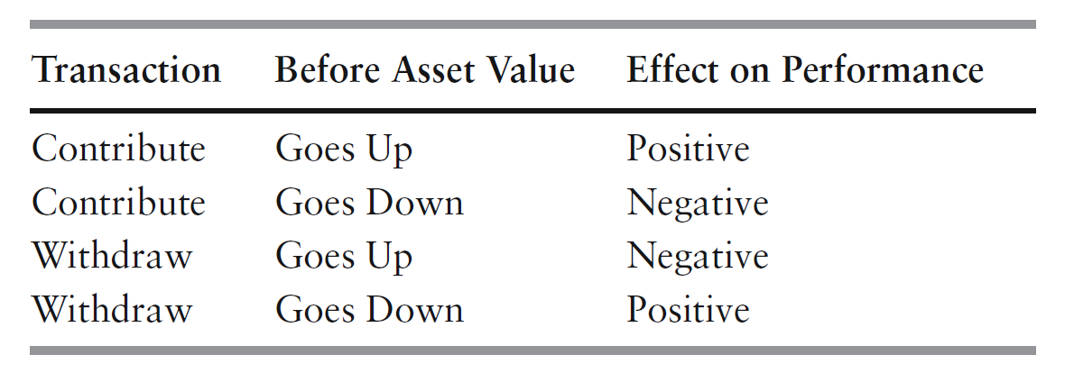
• The timing of [the investor’s] decisions to contribute to or withdraw money from [the portfolio]⁶, with the different cases being summarized in Figure 1, taken from Feibel⁶.

  

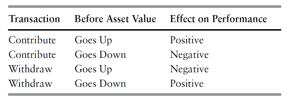
  Figure 1. Impact of external cash flows on money-weighted portfolio performances. Source: Feibel.

Calculation

To borrow a methodology used throughout finance¹, the money-weighted return of a portfolio corresponds to the internal rate of return (IRR) of that portfolio, defined as the rate of return which reconciles the beginning market value and additional cash flows into the portfolio to the ending market value⁶.

Internal rate of return method

Mathematically, the calculation of the (annualized) money-weighted return $r_{mw,irr}$ of a portfolio over a time period through the IRR method is done by solving what is usually called the IRR equation⁷.

Using the notations of this section, that equation is:

\[V_1 - \sum_{i=1}^{T} \frac{C_i}{ \left(1 + r_{mw,irr}\right)^{yearfrac(t_i, t_1)}} - \frac{V_T}{ \left(1 + r_{mw,irr}\right)^{yearfrac(t_T, t_1)}} = 0\]

, where $yearfrac$ is the number of (fractional) years between two dates using a given day count convention.

Numerically, the IRR equation is usually solved by an iterative algorithm, like the Newton-Raphson method or similar other methods.

Modified Dietz method

The calculation of $r_{mw,irr}$ described in the previous sub-section was a problem when computer CPU time was very expensive and needed to be conserved¹, which led to the development of various IRR estimation techniques that did not require [an] iterative algorithm¹.

One of these approximations - the modified Dietz method - is a first-order [closed-form] linear approximation to the IRR¹ method and is the most common⁸ way of calculating periodic investment returns¹.

Mathematically, the calculation of the (total) money-weighted return $r_{mw,md}$ of a portfolio over a time period through the modified Dietz method is done by incorporating “weighted” external cash flows into the formula of the simple rate of return.

Using the notations of this section, this gives:

\[r_{mw,md} = \frac{V_T - V_1 - \sum_{i=1}^T C_i}{V_1 + \sum_{i=1}^T \left( 1 - \frac{yearfrac(t_1, t_i)}{yearfrac(t_1, t_T)} \right) C_i }\]

, where the terms $ 1 - \frac{yearfrac(t_1, t_i)}{yearfrac(t_1, t_T)} $, $i=1..T$, are used to weight the [external cash] flows by the number of days they were available for investment during the period¹.

Caveats

The two money-weighted return calculation methods discussed in the previous sub-sections have certain limitations to be aware of:

• The IRR method provides no theoretical guarantee in general⁹ as to the existence or the unicity of an internal rate of return.

  Indeed, the IRR equation might not have any solution or might have several solutions¹⁰.

  In addition, even when the IRR equation has a unique solution, it might be numerically very hard to find…

• The modified Dietz method has its own issues, for example the accuracy of the result [being] dependent on relatively small capital flows, low volatility and frequent valuations¹¹.

  In particular, a very important point of attention is that the modified Dietz [method] is less useful as an approximation to [IRR] over longer time periods¹.

When to use it?

Calculating the money-weighted return of a portfolio allows to answer the question

How much did a specific investor’s portfolio grow, thanks to both its underlying strategy and its pattern of external cash flows?

Thus, the money-weighted return of a portfolio is an appropriate measure of portfolio performance when it is desired to:

• Compute the rate of return earned on a specific portfolio
• Compare the rate of return earned on a specific portfolio to another rate (rate of inflation, rate of return earned on another portfolio¹², rate of return earned on an alternative investment like real estate or private equity…)
• Analyse the pattern of external cash flows for a specific portfolio¹³

Time-weighted return

The time-weighted return of a portfolio is a form of total return that measures the performance […] for the complete measurement period⁶ in a way that fully eliminates the timing effect that external portfolio cash flows have⁶.

So, contrary to its money-weighted counterpart, the time-weighted return of a portfolio measures only the effects of the market and manager decision⁶.

As a side note, the time-weighted return of a portfolio is the only well-behaved rate of return that is not influenced by contributions or withdrawals², c.f. for example Gray and Dewar².

Calculation

The calculation of the time-weighted return of a portfolio over a time period is easily done through the unit price or unitised method¹, described in Bacon¹:

A standardised unit price or “net asset value” price is calculated immediately before each external cash flow by dividing the market value by the number of units previously allocated. Units are then added or subtracted (bought or sold) in the portfolio at the unit price corresponding to the time of the cash flow […].

Mathematically, using the notations of this section, let be $U_i$, $i=1..T$, corresponding to the following transformation¹⁴ of $V_i$, $i=1..T$:

\[U_1 = 1 \newline U_{i+1} = U_i \frac{V_{i+1}}{V_i + C_i}, i=1..T-1\]

The (total) time-weighted return $r_{tw}$ of the portfolio over the time period $1..T$ is then defined as the simple rate of return of the transformed portfolio values $U_i$, $i=1..T$:

\[r_{tw} = \frac{U_T - U_1}{U_1} = \frac{U_T}{U_1} - 1\]

Caveats

The time-weighted return has two main limitations to be aware of:

• One is practical, with Feibel⁶ noting that there is […] a potentially significant hurdle to implementing this method: the time-weighted return methodology requires valuation of the portfolio before each cash flow⁶.

  For an individual investor, and depending on the exact tools used, this might or might not be a real issue though.

• One is methological, with the time-weighted return of a portfolio being sometimes positive while the overall portfolio is at a loss¹⁵!

  Bacon¹ and Febeil⁶ provide examples of such cases, the bottom line being that it is important [for the portfolio manager] to perform well in the […] period[s] when the majority of client money is invested¹ with the time-weighted return calculation.

When to use it?

Calculating the time-weighted return of a portfolio allows to answer the question

How much did a specific investor’s portfolio grow thanks to its underlying strategy (asset allocation, exposure…)?.

The time-weighted return of a portfolio is thus an appropriate measure of portfolio performance when it is desired to compar[e] the performance of [a portfolio with] different asset managers […] and with benchmark indexes¹.

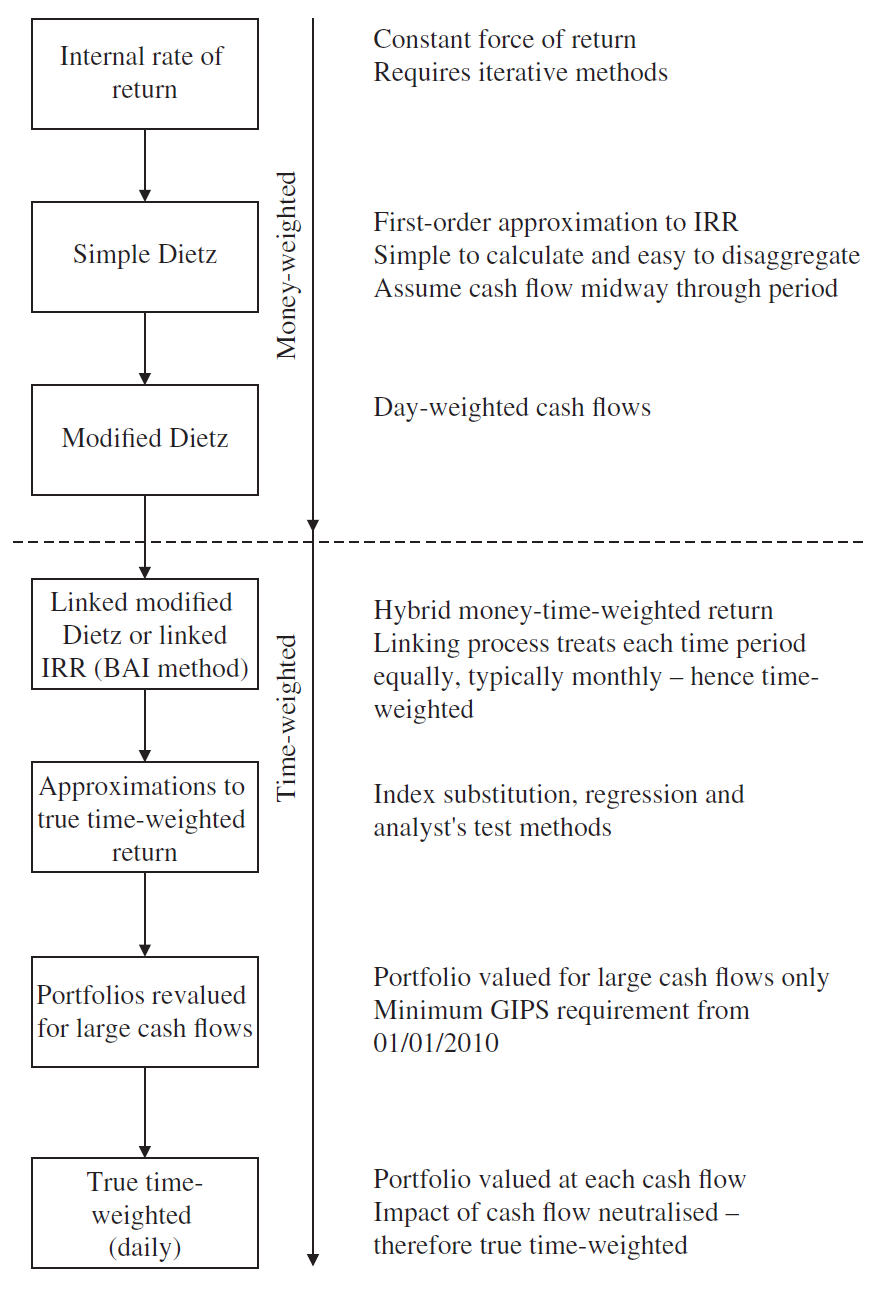
Hybrid return

Bacon¹ notes that in practice, many asset managers use neither true time-weighted nor money-weighted calculations exclusively but rather a hybrid combination of both¹, some of which are depicted in Figure 2, taken from Bacon¹.

Figure 2. The evolution of performance returns methodologies. Source: Bacon.

Money-weighted v.s. time-weighted return

To conclude this section, Figure 3, taken from Feibel⁶, summarizes the respective properties of money-weighted and time-weighted returns.

Figure 3. Properties of money-weighted and time-weighted returns. Source: Feibel.

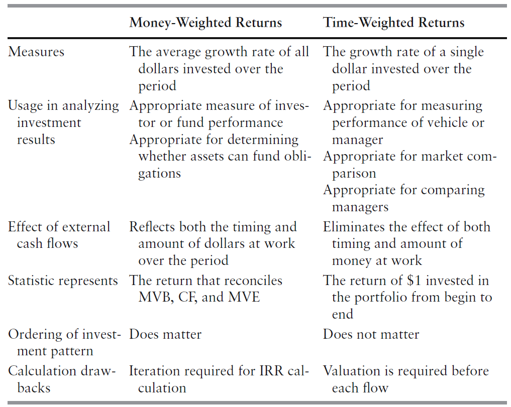
To that summary, I would add that for an individual investor, comparing the money-weighted return and the time-weighted return of a portfolio allows to determine whether the timing of contributions and withdrawals has been successful ($r_{mw} \geq r_{tw}$) or not ($r_{mw} \leq r_{tw}$).

In the latter case, it might be interesting to review¹⁶ the external cash flows timing strategy (panic sells, fomo buys…).

Implementation in Portfolio Optimizer

Portfolio Optimizer allows to:

• Compute the money-weighted and the time-weighted return of a portfolio over a time period, through the endpoints /portfolios/analysis/return/money-weighted and /portfolios/analysis/return/time-weighted.
• Transform portfolio values impacted by external cash flows into money-weighted or time-weighted portfolio values directly usable to compute portfolio performance indicators (return, Sharpe ratio, maximum drawdown…), through the endpoints /portfolios/transformation/money-weighted and /portfolios/transformation/time-weighted.

Examples of usage

I propose to illustrate the differences between money-weighted returns and time-weighted returns through two examples:

• Comparing a dollar cost averaging investment strategy in an ETF to a lump sum investment strategy in the same ETF
• Comparing the returns of an ETF to the returns of an “average” investor in that ETF

Dollar cost averaging v.s. lump sum investing in an MSCI World ETF

Let’s suppose that we would like to compare two investment strategies in the Amundi MSCI World UCITS ETF - EUR (C) over the period 29/12/2023 - 31/12/2024:

• Dollar cost averaging (DCA) investing
  • Portfolio creation - 1000€ on 29/12/2023
  • Portfolio contributions - 100€ at each month’s end
• Lump sum (LS) investing
  • Portfolio creation - 2200€ on 29/12/2023
  • Portfolio contributions - n/a

In both cases, the amount of external portfolio cash flows is the same¹⁷ - equal to 2200€ - but the patterns of these cash flows are different, leading to different portfolio returns:

Portfolio return measure	Total return (%)
Simple return (DCA)	161.42%
Money-weighted return (DCA)	25.45%
Time-weighted return (DCA)	26.33%
Simple return (LS)	26.33%
Money-weighted return (LS)	26.33%
Time-weighted return (LS)	26.33%

Notes:

• Detailed calculations are available in the Google Sheet associated to this blog post.

The table above empirically confirms that:

• In the absence of external cash flows, all portfolio return measures discussed in this blog post become equal (lines #4-#6)
• In the presence of external cash flows

  • The simple return is not an appropriate measure of portfolio return (line #1)

    Despite this, and at the date of publication of this blog post, there are still some financial services using that measure to compute portfolio returns in the presence of external cash flows, like Trading 212, c.f. the associated discussion on their forum.

    Usually, it is because of data availability problems like difficulties in identifying external cash flows, but sometimes it is simply because providing accurate portfolio performance measures is not a priority…

  • The money-weighted return is impacted by the timing of external cash flows (line #2)

    Here, there is a ~-1% difference between the portfolio money-weighted and time-weighted returns, mainly due to the ill-timed¹⁸ contribution made on 28/03/2024.

    Such a difference is relatively insignificant over one year, but depending on the pattern of external cash flows, it could be much worse.

    For example, if a unique contribution of 1200€ on 28/03/2024 was made instead of monthly contributions of 100€, the associated portfolio money-weighted return would decrease to 22.59%, representing this time a ~-4% difference!

  • The time-weighted return is not impacted by external cash flows¹⁹ and is akin to a “lump sum investing”-equivalent return (line #3 is equal to lines #4-#6)

Investment returns v.s. average investor returns in an MSCI World ETF

Financial studies regularly show that investors tend to lag actual fund returns across a variety of asset classes, leading to what is usually called the investor gap²⁰²¹.

For example:

• The Dalbar’s Quantitative Analysis of Investor Behavior (QAIB) annual study measure[s] the effects of investor decisions to buy, sell and switch into and out of funds over short and long-term timeframes²² and the results consistently show that the average investor earns less – in many cases, much less – than mutual fund performance reports would suggest²².

  For the U.S., Figure 4, adapted from Dalbar²², depicts the returns of U.S. funds v.s. the returns of the average investor in U.S. funds over the period 1994-2023.

  

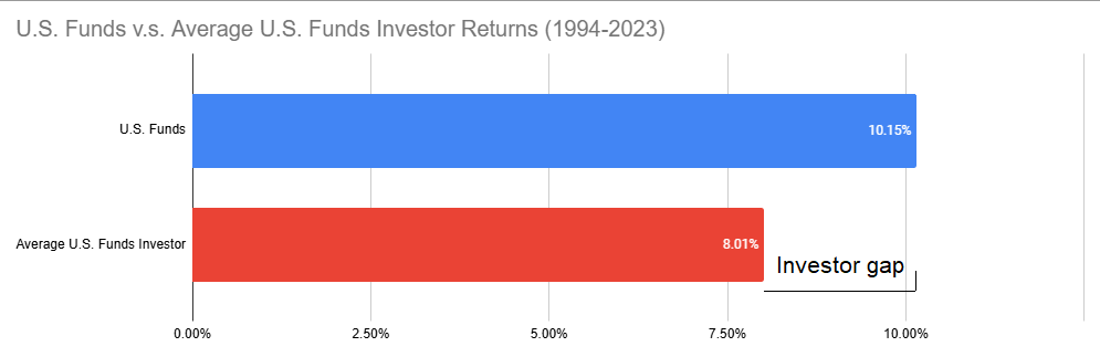
  Figure 4. U.S. funds returns v.s. average U.S. funds investor returns (30-year returns, 1994-2023). Source: Dalbar.

  The observed performance differencial of ~2% per year creates dramatic cumulative effects over such a long period²²!

• The Morningstar’s Mind the Gap annual study compares funds’ dollar-weighted returns [- that is, funds’ returns as experienced by their investors -] with their time-weighted returns to see how large the gap, or difference, has been over time²³ and analyses where investors succeeded in capturing most of their funds’ returns²³.

  Figure 5, directly taken from Morningstar²³, illustrates that gap by U.S. funds category over the 10 years ended 31th December 2023.

  

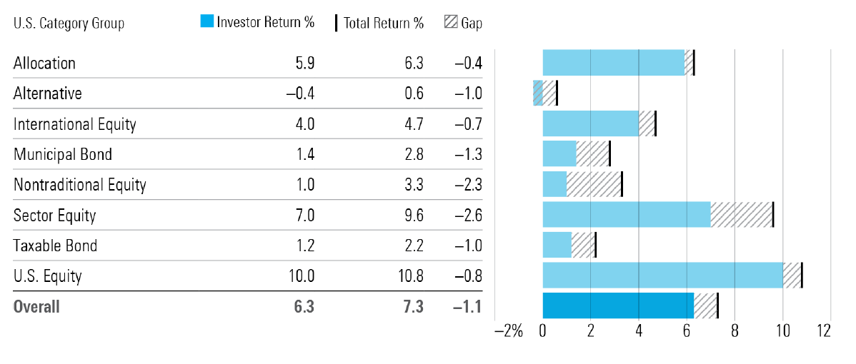
  Figure 5. Investor return gaps by U.S. category group (10-year returns, 2013-2023). Source: Morningstar.

In this sub-section, I propose to apply the same methodology as these studies to the Amundi MSCI World UCITS ETF - EUR (C) over the period 30/04/2018 - 31/12/2024.

In more details:

• I will use the month-end asset data [(AUM)] compared with the underlying total return to estimate a net inflow or outflow for [each] month²³, using Morningstar’s approach to estimating funds’ monthly net flows²⁴:

  The [net] cash flow estimate for a month $C_t$ is the difference in the beginning $NAV_{t-1}$ and ending $NAV_t$ total net assets that cannot be explained by the monthly total return $r_t$, that is, $ C_t = NAV_t - NAV_{t-1} \left( 1 + r_t \right) $.

• Once all the monthly cash flows are available for the period²³, I will calculate the associated money-weighted return - which correspond to the average investor return in the ETF - and I will then compare it to the ETF money-weighted return²⁵ - which corresponds to the ETF return itself.

Notes:

• Detailed calculations are available in the Google Sheet associated to this blog post.

Results are the following:

Portfolio return measure	Annualized return (%)
Money-weighted return (AUM)	14.15%
Time-weighted return (AUM)	12.74%

The table above confirms the presence of an investor gap for the considered MSCI World ETF, but for once, to the benefit (of around ~1.5% yearly) of the average investor!

This is at odds with Morningstar’s findings²³ that the gap between index ETFs’ dollar-weighted returns and their total return […] was quite a bit wider than the gap for index open-end funds²³, but of couse, the analysis of this sub-section has no statistical significance compared to that of Morningstar.

Or, maybe investors in the Amundi MSCI World UCITS ETF have specific timing abilities, who knows!

Conclusion

As mentioned in the introduction, the calculation of portfolio return is the first step in the performance measurement process¹.

Once properly done, the next step is to know if the return is good or bad. In other words, [it is needed] to evaluate performance (risk and return), against an appropriate benchmark¹, which can for example be random portfolios.

For more discussions on portfolio performances, feel free to connect with me on LinkedIn or to follow me on Twitter.

–

1. See Carl Bacon, Practical Portfolio Performance Measurement and Attribution, Third edition. ↩ ↩² ↩³ ↩⁴ ↩⁵ ↩⁶ ↩⁷ ↩⁸ ↩⁹ ↩¹⁰ ↩¹¹ ↩¹² ↩¹³ ↩¹⁴ ↩¹⁵ ↩¹⁶ ↩¹⁷ ↩¹⁸ ↩¹⁹ ↩²⁰ ↩²¹ ↩²² ↩²³

2. See Kenneth B. Gray, Jr. and Robert B. K. Dewar, Axiomatic Characterization of the Time-Weighted Rate of Return, Management Science, Vol. 18, No. 2, Application Series (Oct., 1971), pp. B32-B35. ↩ ↩² ↩³ ↩⁴ ↩⁵

3. See W. Marty, Portfolio Analytics. An Introduction to Return and RiskMeasurement, Springer Texts in Business and Economics (2nd edition), Springer Berlin, 2015.. ↩

4. Internal cash flows our of the portfolio is sometimes refered to as income¹⁶ from the portfolio constituents. ↩

5. In contrast with the price return of the portfolio, which would only take into account the price evolution of the portfolio constituents. ↩

6. See Bruce J. Feibel, Investment Performance Measurement. ↩ ↩² ↩³ ↩⁴ ↩⁵ ↩⁶ ↩⁷ ↩⁸ ↩⁹ ↩¹⁰ ↩¹¹ ↩¹² ↩¹³ ↩¹⁴ ↩¹⁵ ↩¹⁶ ↩¹⁷

7. As noted in Bacon¹, the formal definition of the IRR is the discount rate that makes the net present value equal to zero in a discounted cash flow analysis¹; that equation is precisely the equation of the net present value in the specific case of a portfolio of assets. ↩

8. For example, the modified Dietz method is used in Interactive Brokers PortfolioAnalyst product to compute the money-weighted return of the investor’s portfolio. ↩

9. C.f. for example the documentation of the Excel’s function XIRR. ↩

10. Although Bacon¹ notes that you need to work very hard, with quite extreme data, to generate suitable examples¹ because multiple solutions are extremely unlikely to be experienced in practice¹. ↩

11. See Hager DP. Measurement of Pension Fund Investment Performance. Journal of the Staple Inn Actuarial Students’ Society. 1980;24:33-64. ↩

12. For Bacon¹, though, the money-weighted return is unique and not really comparable with other portfolios enjoying a different pattern of cash flow¹; on this, I kindly disagree, because as an individual investor, I will for example certainly be pleased to have a higher money-weighted return than that of my father/brother in law! ↩

13. For example when testing for investor’s skill in timing external cash flows or when comparing dollar-cost averaging (DCA) investment strategies (weekly, monthly, quarterly…). ↩

14. That transformation is in effect a normalised market value¹ transformation of the portfolio. ↩

15. Or conversely, with the time-weighted return of a portfolio being sometimes negative while the overall portfolio is at a gain!! ↩

16. For example, by switching to a dollar cost averaging strategy. ↩

17. The last contribution of 100€ made on 31/12/2024 is excluded from this count, since it is invested at the end of the considered period. ↩

18. From 28/03/2024 to 30/04/2024, the MSCI World ETF under consideration returned -2.74%. ↩

19. The time-weighted return is also equal to the NAV return. ↩

20. To be noted that the investor gap as discussed here is not related to fund fees; for example, Morningstar²³ didn’t find a strong link between fees and investor return gaps in the study²³. ↩

21. Also known as the behaviour gap. ↩

22. See Dalbar’s 2024 QAIB Report. ↩ ↩² ↩³ ↩⁴

23. See Morningstar’s Mind the Gap 2024 Report. ↩ ↩² ↩³ ↩⁴ ↩⁵ ↩⁶ ↩⁷ ↩⁸ ↩⁹

24. See Morningstar’s Estimated Net Cash Flow Methodology. ↩

25. As with most funds, ETF returns correspond to time-weighted returns. ↩