More Bootstrap Simulations with Portfolio Optimizer: the Autoregressive Online Bootstrap

7 minute read

In a previous article, I described several classical bootstrap techniques — i.i.d. bootstrap, circular block bootstrap, and stationary block bootstrap — and showed how the stationary block bootstrap could be used to simulate future price paths for financial assets by following the methodology of Anarkulova et al.¹.

In this blog post, I will detail another bootstrap technique called the autoregressive online bootstrap² and introduced in Palm and Nagler², that is best described as a multiplier bootstrap³ coupled with an autoregressive sequence of weights specifically chosen to make it useable with streaming time series data.

As an example of usage, I will simulate alternative price histories for the SPY and TLT ETFs, which are ETFs representative of the US stock market and of the long-term US Treasury bonds.

Mathematical preliminaries

Let $X_1, …, X_n$⁴, $n \geq 1$ be a sample of data observed from a population.

Limitations of classical bootstrap techniques in an online setting

In a typical⁵ online setting, the length $n$ of the sample of data $X_1, …, X_n$ is growing infinitely, with new events [that] are observed at the moment they occur².

In such a setting, the classical bootstrap techniques described in the previous blog post on bootstrap simulations require all data observed so far² at any given point in time.

Indeed:

The i.i.d. bootstrap, by definition, requires keeping track of the entire observed sample $ {X_1, …, X_n} $².
The circular and the stationary block bootstrap require all blocks […] to increase in size with $n$², so that to compute the bootstrap in practice, the entire data set $ {X_1, …, X_n} $ needs to be kept in memory and processed fully, every time the block size changes².

Depending on the domain of application, this can be a serious computational limitation when:

n is large
n is moderately large but the underlying $n$ observations require a lot of computer memory to be stored
n is moderately large but the computation time is limited (e.g. real-time applications)

The multiplier bootstrap

The multiplier bootstrap³ is a general class of bootstrapping schemes based on perturbations of the original observations with suitable weights².

In other words, compared to classical bootstrap techniques, the multiplier bootstrap replaces the idea of “randomly resampling observations” with the idea of “randomly reweighting observations”, which enables it to be applied in an online setting.

For i.i.d. data $X_1, …, X_n$, it is defined as follows:

Let $V_1, …, V_n$ be $n$ i.i.d. random variables of unit mean/variance.
Let $ \bar V_i = \frac{1}{i} \sum_{j=1}^{i} V_j $ the running mean of these random variables, which can be computed recursively through the formula
\[\bar V_i = \frac{(i-1) \bar V_{i-1} + V_i }{i}\]
The multiplier bootstrap samples $ X_1^*,…,X_n^* $ are then defined as
\[X_i^* = \frac{V_i}{\bar V_i} X_i\]

The autoregressive online bootstrap

Methodology

The autoregressive online bootstrap² is a specific instance of the multiplier bootstrap that generates a sequence of random weights evolving according to an autoregressive process centered around 1:

\[V_i = 1 + \rho_i \left( V_{i-1} - 1 \right) + \sqrt{1 - \rho_i^2} \zeta_i, i=1..n\]

, with:

$V_0 = 0$
$\rho_i = 1 - i^{-\beta}$, $ 0 < \beta < \frac{1}{2}$
$\zeta_i \sim \mathcal N(0,1), i=1..n$

The associated autoregressive online bootstrap samples $ X_1^*,…,X_n^* $ are then defined as

\[X_i^* = \frac{V_i}{\bar V_i} X_i\]

Rationale

Palm and Nagler² notes that for the multiplier bootstrap to remain valid for time series:

The dependencies between weights $V_i$ and $V_j$ must increase with the sample size $n$, but at the same time remain almost independent when the time gap $|i-j|$ is sufficiently large compared to $n$².
A scaling of the weights by their arithmetic mean is also necessary²

This is what they propose with the autoregressive online bootstrap technique.

Properties

The main result of Palm and Nagler² is that under mild conditions on the original data $X_1, …, X_n$, the autoregressive online bootstrap is a consistent resampling scheme for the mean and for any continously differentiable transformation of the mean⁶ of an univariate or a multivariate time series.

How to select the parameter $\beta$?

The parameter $\beta$ controls the behaviour of the autoregressive online bootstrap samples in a way similar to how the block length controls the behaviour of the block bootstrap samples in classical block bootstrap techniques.

Intuitively:

A small value of $\beta$ leads to slowly changing weights and thus to long stretches of bootstrap samples that are consistent with the original observations, although up- or down-weighted.

This is similar in spirit to having a long block size in a block bootstrap technique.
On the contrary, a large value of $\beta$ leads to quickly changing weights and thus to rapidly varying bootstrap samples.

This is similar in spirit to having a short block size in a block bootstrap technique.

Palm and Nagler² demonstrates that $\beta_{opt} = \sqrt{2} - 1$ allows for an optimal bias-variance trade-off², so that unless there is a specific need to play with this parameter, using that value should be the default choice.

Practical performances

Palm and Nagler² compares the practical performances of the autoregressive online bootstrap to an i.i.d. multiplier bootstrap and to a block bootstrap technique called the moving average block bootstrap⁷.

In particular, Palm and Nagler² shows that:

The two time series bootstraps achieve approximately correct coverage in all [studied] scenarios, even in the presence of nonlinear [AR(2)-GARCH(1,1)] dependencies² corresponding to a stochastic volatility process.
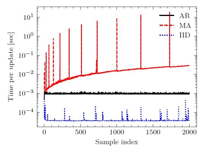
The autoregressive online bootstrap allows for cheap online updates - in constant time, as illustrated in Figure 1 - contrary to the moving average block bootstrap.

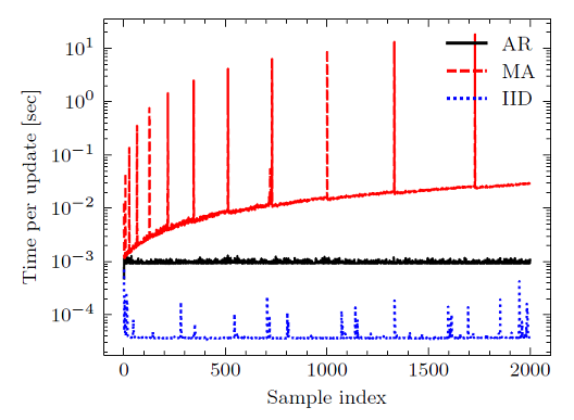
Figure 1. Computation time per online update of 200 bootstrap samples as the bootstrap techniques progress through a stream of 2000 samples. Source: Palm and Nagler.
The autoregressive online bootstrap has a slightly higher variance compared to the moving average block bootstrap, which is the cost [to] pay for its computational advantage².

Caveats

One important limitation of the autoregressive online bootstrap is that the weights $V_i$,$i=1..n$ can be negative.

For this reason, in finance, logarithmic asset returns should then be prefered to either asset prices (since they could become negative) or arithmetic asset returns (singe they could become < -100%).

Implementations

Implementation in Portfolio Optimizer

Portfolio Optimizer implements the autoregressive online bootstrap through the endpoint /assets/returns/simulation/bootstrap/online.

Implementation elsewhere

An implementation of the autoregressive online bootstrap in Python is available at https://github.com/nicolaipalm/online-bootstrap-implementation by its authors.

Example of usage - Simulation of alternative price histories for ETFs

As an example of usage, I propose to use the autoregressive online bootstrap to generate alternative price histories for the SPY and TLT ETFs and compute a couple of associated descriptive statistics⁸.

Alternative price histories for the SPY ETF

Figure 2 illustrates 10 synthetic price histories generated by applying the autoregressive online bootstrap to the logarithmic returns of the SPY ETF over the period 1st January 2025 - 31th December 2025⁹.

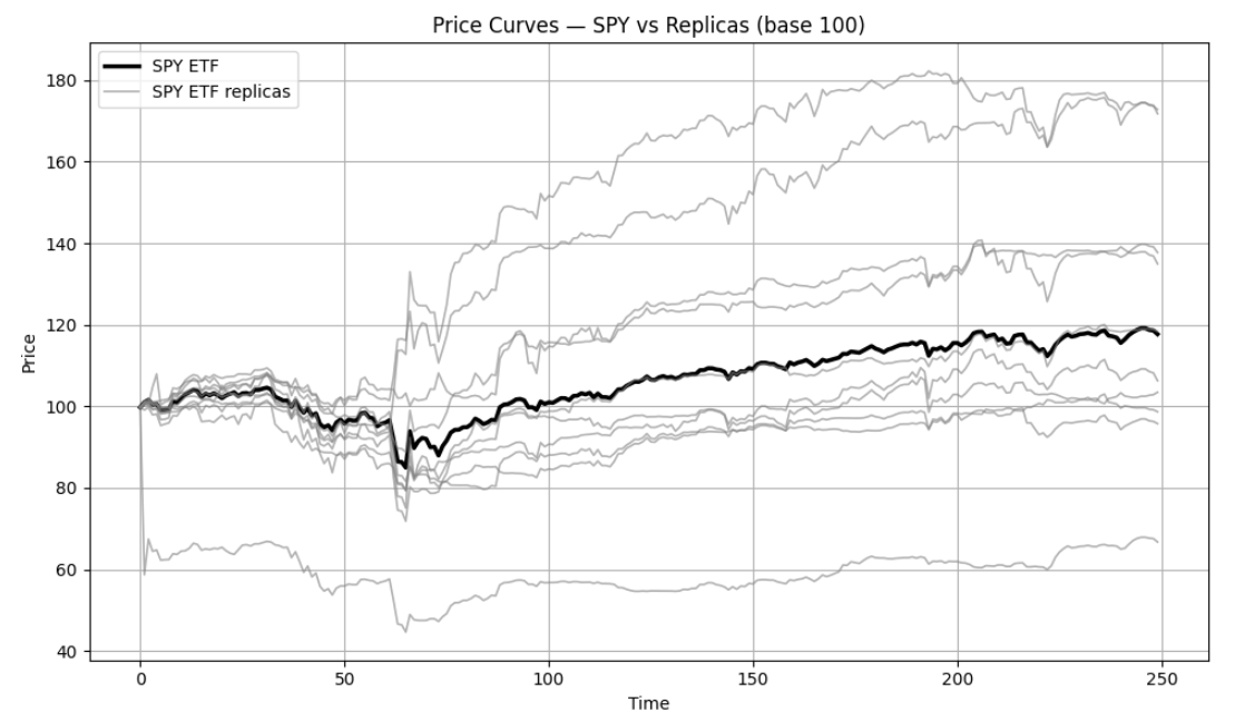
On Figure 2, it is visible that the autoregressive online bootstrap allows for a wide variety of scenarios to be generated.

This is confirmed in Figure 3, which depicts the distributions of the first four moments of the logarithmic returns of 1000 synthetic price histories generated by applying the autoregressive online bootstrap to the logarithmic returns of the SPY ETF over the period 1st January 2025 - 31th December 2025⁹.

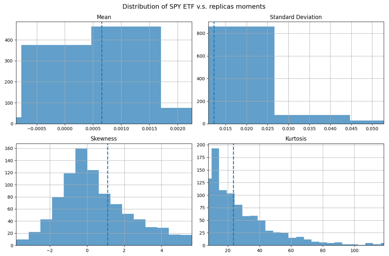
Figure 3. Distributions of the first four moments of 1000 alternative price histories for the SPY ETF, autoregressive online bootstrap, 1st January 2025 - 31th December 2025.

Figure 3 empirically demonstrates two points:

It confirms the mean-preservation property of the autoregressive online bootstrap.

As a side note, in case this is a problem for the usage at hand, it is always possible to alter the mean of the generated scenarios in a perfectly controlled way, c.f. a previous blog post.
It shows that the autoregressive online bootstrap can generate scenarios with a wildly different standard deviation/skewness/kurtosis compared to the original one.

Here, to be noted that some scenarios might seem implausible, with a kurtosis > 100 for example.

Nevertheless, implausible does not equal impossible¹⁰, so that depending on the usage at hand, such scenarios could be eliminated or put aside for specific stress-testing.

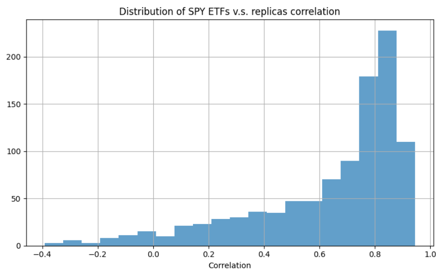
Figure 4 illustrates the variety of scenarios in another way, by looking at the correlation between the logarithmic returns of the SPY ETF and of its 1000 alternatives, which approximatively ranges from -0.4 to 1.

Figure 4. Distribution of the correlation between the SPY ETF price history and 1000 alternative price histories, autoregressive online bootstrap, 1st January 2025 - 31th December 2025.

Alternative price histories for the SPY and TLT ETFs

Figure 5 illustrates the behaviour of the autoregressive online boostrap in terms of bivariate correlation when applied to the logarithmic returns of both the SPY and TLT ETFs over the period 1st January 2025 - 31th December 2025⁹.

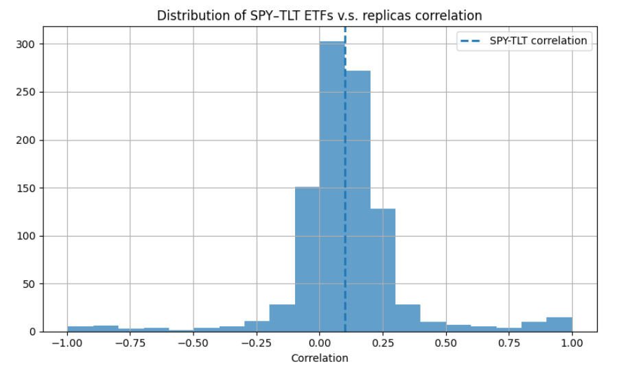
From Figure 5, it appears that the whole range of admissible correlations $[-1,1]$ is achievable through the autoregressive online bootstrap, with the majority of scenarios falling in the interval $[-0.25, 0.50]$.

Conclusion

The autoregressive online bootstrap introduced in Palm and Nagler² and detailled in this blog post provides an alternative to classical block bootstrap techniques for time series that is specifically taylored to streaming data.

Don’t hesitate to experiment with it and evaluate whether it could replace your current boostrap methodology!

As usual, feel also free to connect with me on LinkedIn or to follow me on Twitter.

–

See Anarkulova, Aizhan and Cederburg, Scott and O’Doherty, Michael S., The Long-Horizon Returns of Stocks, Bonds, and Bills: Evidence from a Broad Sample of Developed Markets (November 15, 2021). ↩
See Nicolai Palm, Thomas Nagler; An Online Bootstrap for Time Series; Proceedings of The 27th International Conference on Artificial Intelligence and Statistics, PMLR 238:190-198. ↩ ↩² ↩³ ↩⁴ ↩⁵ ↩⁶ ↩⁷ ↩⁸ ↩⁹ ↩¹⁰ ↩¹¹ ↩¹² ↩¹³ ↩¹⁴ ↩¹⁵ ↩¹⁶ ↩¹⁷ ↩¹⁸ ↩¹⁹ ↩²⁰
See Van Der Vaart, A. W. and Wellner, J. A. Weak convergence. In Weak convergence and empirical processes, pp. 16–28. Springer, 1996. ↩ ↩²
The observations $X_1, …, X_n$ can be observations of random variables or of random vectors. ↩
It is also possible that for computational reasons - like a huge $n$ - a complete data set is available from the start², but is processed sequentially or in batches². ↩
Like the variance, c.f. Palm and Nagler². ↩
See Buhlmann, P. L. (1993). The blockwise bootstrap in time series and empirical processes. PhD thesis, ETH Zurich. ↩
In practice, the generation of such alternative price histories would typically be integrated into a backtesting engine. ↩
(Adjusted) prices of the SPY and TLT ETFs have have been retrieved using Tiingo. ↩ ↩² ↩³
Who could have predicted the price action of gold and silver on 30th January 2026? ↩